在圖片處理中，霍夫變換主要是用來檢測圖片中的幾何形狀，包括直線、圓、橢圓等。

在skimage中，霍夫變換是放在tranform模組內，本篇主要講解霍夫線變換。

對於平面中的一條直線，在笛卡爾座標系中，可用y=mx+b來表示，其中m為斜率，b為截距。但是如果直線是一條垂直線，則m為無窮大，所有通常我們在另一座標系中表示直線，即極座標系下的r=xcos(theta)+ysin(theta)。即可用（r,theta）來表示一條直線。其中r為該直線到原點的距離，theta為該直線的垂線與x軸的夾角。如下圖所示。

對於一個給定的點（x0,y0), 我們在極座標下繪出所有通過它的直線（r,theta)，將得到一條正弦曲線。如果將圖片中的所有非0點的正弦曲線都繪製出來，則會存在一些交點。所有經過這個交點的正弦曲線，說明都擁有同樣的(r,theta), 意味著這些點在一條直線上。

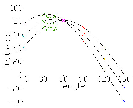
發上圖所示，三個點(對應圖中的三條正弦曲線）在一條直線上，因為這三個曲線交於一點，具有相同的（r, theta)。霍夫線變換就是利用這種方法來尋找圖中的直線。

函式：skimage.transform.hough_line(img)

返回三個值：

h: 霍夫變換累積器

theta: 點與x軸的夾角集合，一般為0-179度

distance: 點到原點的距離，即上面的所說的r.

例：

import skimage.transform as st
import numpy as np
import matplotlib.pyplot as plt

# 構建測試圖片
image = np.zeros((100, 100))  #
 
背景圖
idx = np.arange(25, 75)    #25-74序列
image[idx[::-1], idx] = 255  # 線條\
image[idx, idx] = 255        # 線條/

# hough線變換
h, theta, d = st.hough_line(image)

#生成一個一行兩列的視窗（可顯示兩張圖片）.
fig, (ax0, ax1) = plt.subplots(1, 2, figsize=(8, 6))
plt.tight_layout()

#顯示原始圖片
ax0.imshow(image, plt.cm.gray)
ax0.set_title(
 
'Input image')
ax0.set_axis_off()

#顯示hough變換所得資料
ax1.imshow(np.log(1 + h))
ax1.set_title('Hough transform')
ax1.set_xlabel('Angles (degrees)')
ax1.set_ylabel('Distance (pixels)')
ax1.axis('image')

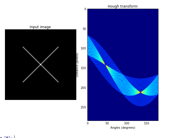
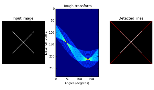
從右邊那張圖可以看出，有兩個交點，說明原影象中有兩條直線。

如果我們要把圖中的兩條直線繪製出來，則需要用到另外一個函式：

skimage.transform.hough_line_peaks(hspace, angles, dists）

用這個函式可以取出峰值點，即交點，也即原圖中的直線。

返回的引數與輸入的引數一樣。我們修改一下上邊的程式，在原圖中將兩直線繪製出來。

import skimage.transform as st
import numpy as np
import matplotlib.pyplot as plt

# 構建測試圖片
image = np.zeros((100, 100))  #背景圖
idx = np.arange(25, 75)    #25-74序列
image[idx[::-1], idx] = 255  # 線條\
image[idx, idx] = 255        # 線條/

# hough線變換
h, theta, d = st.hough_line(image)

#生成一個一行三列的視窗（可顯示三張圖片）.
fig, (ax0, ax1,ax2) = plt.subplots(1, 3, figsize=(8, 6))
plt.tight_layout()

#顯示原始圖片
ax0.imshow(image, plt.cm.gray)
ax0.set_title('Input image')
ax0.set_axis_off()

#顯示hough變換所得資料
ax1.imshow(np.log(1 + h))
ax1.set_title('Hough transform')
ax1.set_xlabel('Angles (degrees)')
ax1.set_ylabel('Distance (pixels)')
ax1.axis('image')

#顯示檢測出的線條
ax2.imshow(image, plt.cm.gray)
row1, col1 = image.shape
for _, angle, dist in zip(*st.hough_line_peaks(h, theta, d)):
    y0 = (dist - 0 * np.cos(angle)) / np.sin(angle)
    y1 = (dist - col1 * np.cos(angle)) / np.sin(angle)
    ax2.plot((0, col1), (y0, y1), '-r')
ax2.axis((0, col1, row1, 0))
ax2.set_title('Detected lines')
ax2.set_axis_off()

注意，繪製線條的時候，要從極座標轉換為笛卡爾座標，公式為：

skimage還提供了另外一個檢測直線的霍夫變換函式，概率霍夫線變換：

skimage.transform.probabilistic_hough_line(img, threshold=10, line_length=5,line_gap=3)

引數：

img: 待檢測的影象。

threshold： 閾值，可先項，預設為10

line_length: 檢測的最短線條長度，預設為50

line_gap: 線條間的最大間隙。增大這個值可以合併破碎的線條。預設為10

返回：

lines: 線條列表, 格式如((x0, y0), (x1, y0))，標明開始點和結束點。

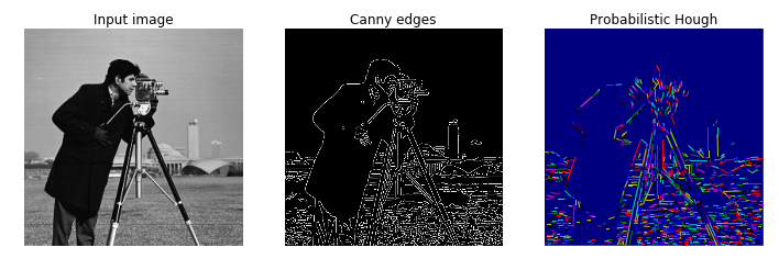
下面，我們用canny運算元提取邊緣，然後檢測哪些邊緣是直線？

import skimage.transform as st
import matplotlib.pyplot as plt
from skimage import data,feature

#使用Probabilistic Hough Transform.
image = data.camera()
edges = feature.canny(image, sigma=2, low_threshold=1, high_threshold=25)
lines = st.probabilistic_hough_line(edges, threshold=10, line_length=5,line_gap=3)

# 建立顯示視窗.
fig, (ax0, ax1, ax2) = plt.subplots(1, 3, figsize=(16, 6))
plt.tight_layout()

#顯示原影象
ax0.imshow(image, plt.cm.gray)
ax0.set_title('Input image')
ax0.set_axis_off()

#顯示canny邊緣
ax1.imshow(edges, plt.cm.gray)
ax1.set_title('Canny edges')
ax1.set_axis_off()

#用plot繪製出所有的直線
ax2.imshow(edges * 0)
for line in lines:
    p0, p1 = line
    ax2.plot((p0[0], p1[0]), (p0[1], p1[1]))
row2, col2 = image.shape
ax2.axis((0, col2, row2, 0))
ax2.set_title('Probabilistic Hough')
ax2.set_axis_off()
plt.show()