
xgboost 實戰以及原始碼分析
1.序
距離上一次編輯將近10個月,幸得愛可可老師(微博)推薦,訪問量陡增。最近畢業論文與xgboost相關,於是重新寫一下這篇文章。
關於xgboost的原理網路上的資源很少,大多數還停留在應用層面,本文通過學習陳天奇博士的PPT、論文、一些網路資源,希望對xgboost原理進行深入理解。(筆者在最後的參考文獻中會給出地址)
2.xgboost vs gbdt
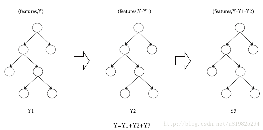
說到xgboost,不得不說gbdt,兩者都是boosting方法(如圖1所示),瞭解gbdt可以看我這篇文章 地址。
如果不考慮工程實現、解決問題上的一些差異,xgboost與gbdt比較大的不同就是目標函式的定義。
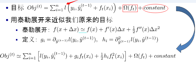
注:紅色箭頭指向的l即為損失函式;紅色方框為正則項,包括L1、L2;紅色圓圈為常數項。xgboost利用泰勒展開三項,做一個近似,我們可以很清晰地看到,最終的目標函式只依賴於每個資料點的在誤差函式上的一階導數和二階導數。
3.原理
對於上面給出的目標函式,我們可以進一步化簡
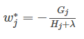
(1)定義樹的複雜度
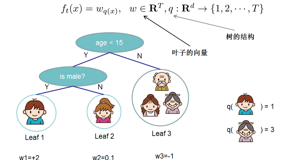
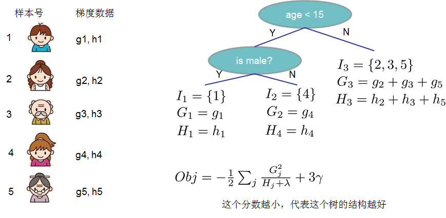
對於f的定義做一下細化,把樹拆分成結構部分q和葉子權重部分w。下圖是一個具體的例子。結構函式q把輸入對映到葉子的索引號上面去,而w給定了每個索引號對應的葉子分數是什麼。
定義這個複雜度包含了一棵樹裡面節點的個數,以及每個樹葉子節點上面輸出分數的L2模平方。當然這不是唯一的一種定義方式,不過這一定義方式學習出的樹效果一般都比較不錯。下圖還給出了複雜度計算的一個例子。
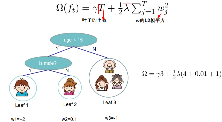
注:方框部分在最終的模型公式中控制這部分的比重,對應模型引數中的lambda ,gamma
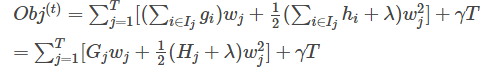
在這種新的定義下,我們可以把目標函式進行如下改寫,其中I被定義為每個葉子上面樣本集合 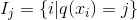
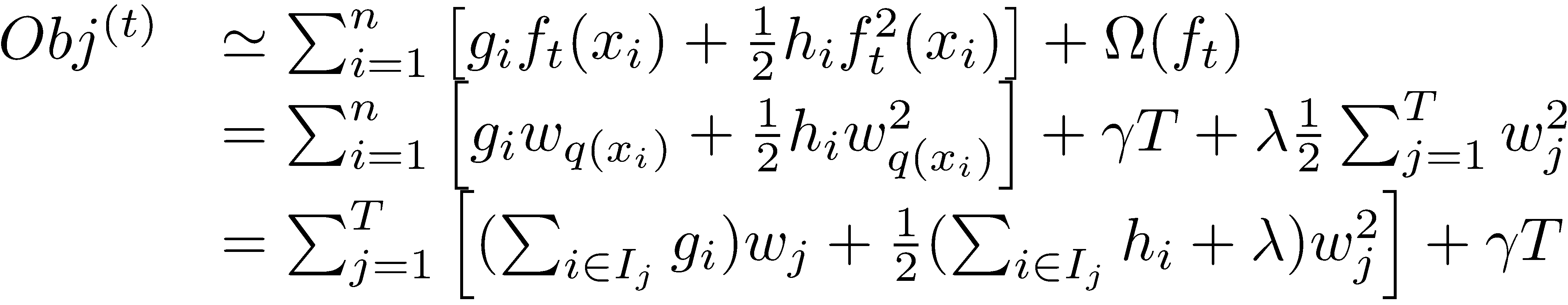
這一個目標包含了T個相互獨立的單變數二次函式。我們可以定義
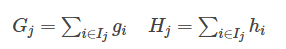
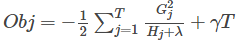
最終公式可以化簡為
通過對
然後把
(2)打分函式計算示例
Obj代表了當我們指定一個樹的結構的時候,我們在目標上面最多減少多少。我們可以把它叫做結構分數(structure score)
(3)分裂節點
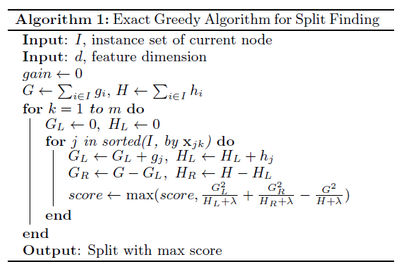
論文中給出了兩種分裂節點的方法
(1)貪心法:
每一次嘗試去對已有的葉子加入一個分割
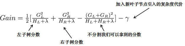
對於每次擴充套件,我們還是要列舉所有可能的分割方案,如何高效地列舉所有的分割呢?我假設我們要列舉所有x < a 這樣的條件,對於某個特定的分割a我們要計算a左邊和右邊的導數和。
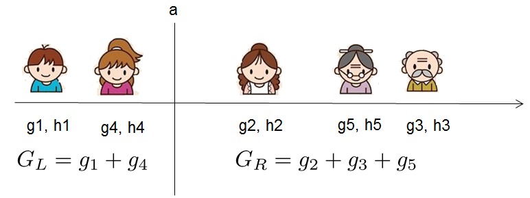
我們可以發現對於所有的a,我們只要做一遍從左到右的掃描就可以枚舉出所有分割的梯度和GL和GR。然後用上面的公式計算每個分割方案的分數就可以了。
觀察這個目標函式,大家會發現第二個值得注意的事情就是引入分割不一定會使得情況變好,因為我們有一個引入新葉子的懲罰項。優化這個目標對應了樹的剪枝, 當引入的分割帶來的增益小於一個閥值的時候,我們可以剪掉這個分割。大家可以發現,當我們正式地推導目標的時候,像計算分數和剪枝這樣的策略都會自然地出現,而不再是一種因為heuristic(啟發式)而進行的操作了。
下面是論文中的演算法
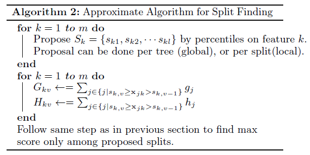
(2)近似演算法:
主要針對資料太大,不能直接進行計算
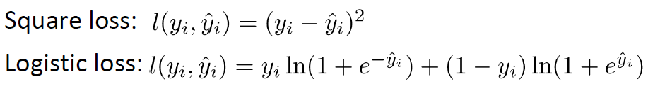
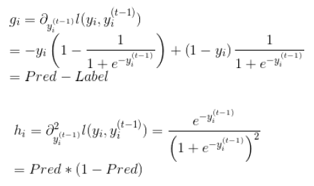
4.自定義損失函式(指定grad、hess)
(1)損失函式
(2)grad、hess推導
(3)官方程式碼
#!/usr/bin/python
import numpy as np
import xgboost as xgb
###
# advanced: customized loss function
#
print ('start running example to used customized objective function')

dtrain = xgb.DMatrix('../data/agaricus.txt.train')
dtest = xgb.DMatrix('../data/agaricus.txt.test')

# note: for customized objective function, we leave objective as default
# note: what we are getting is margin value in prediction
# you must know what you are doing
param = {'max_depth': 2, 'eta': 1, 'silent': 1}
watchlist = [(dtest, 'eval'), (dtrain, 'train')]
num_round = 2

# user define objective function, given prediction, return gradient and second order gradient
# this is log likelihood loss
def logregobj(preds, dtrain):
    labels = dtrain.get_label()
    preds = 1.0 / (1.0 + np.exp(-preds))
    grad = preds - labels
    hess = preds * (1.0-preds)
    return grad, hess

# user defined evaluation function, return a pair metric_name, result
# NOTE: when you do customized loss function, the default prediction value is margin
# this may make builtin evaluation metric not function properly
# for example, we are doing logistic loss, the prediction is score before logistic transformation
# the builtin evaluation error assumes input is after logistic transformation
# Take this in mind when you use the customization, and maybe you need write customized evaluation function
def evalerror(preds, dtrain):
    labels = dtrain.get_label()
    # return a pair metric_name, result
    # since preds are margin(before logistic transformation, cutoff at 0)
    return 'error', float(sum(labels != (preds > 0.0))) / len(labels)

# training with customized objective, we can also do step by step training
# simply look at xgboost.py's implementation of train
bst = xgb.train(param, dtrain, num_round, watchlist, logregobj, evalerror)- 1
- 2
- 3
- 4
- 5
- 6
- 7
- 8
- 9
- 10
- 11
- 12
- 13
- 14
- 15
- 16
- 17
- 18
- 19
- 20
- 21
- 22
- 23
- 24
- 25
- 26
- 27
- 28
- 29
- 30
- 31
- 32
- 33
- 34
- 35
- 36
- 37
- 38
- 39
- 40
- 41
- 42
- 1
- 2
- 3
- 4
- 5
- 6
- 7
- 8
- 9
- 10
- 11
- 12
- 13
- 14
- 15
- 16
- 17
- 18
- 19
- 20
- 21
- 22
- 23
- 24
- 25
- 26
- 27
- 28
- 29
- 30
- 31
- 32
- 33
- 34
- 35
- 36
- 37
- 38
- 39
- 40
- 41
- 42
5.Xgboost調參
由於xgboost的引數過多,這裡介紹三種思路
(3)老外寫的一篇文章,操作性比較強,推薦學習一下。地址
6.工程實現優化
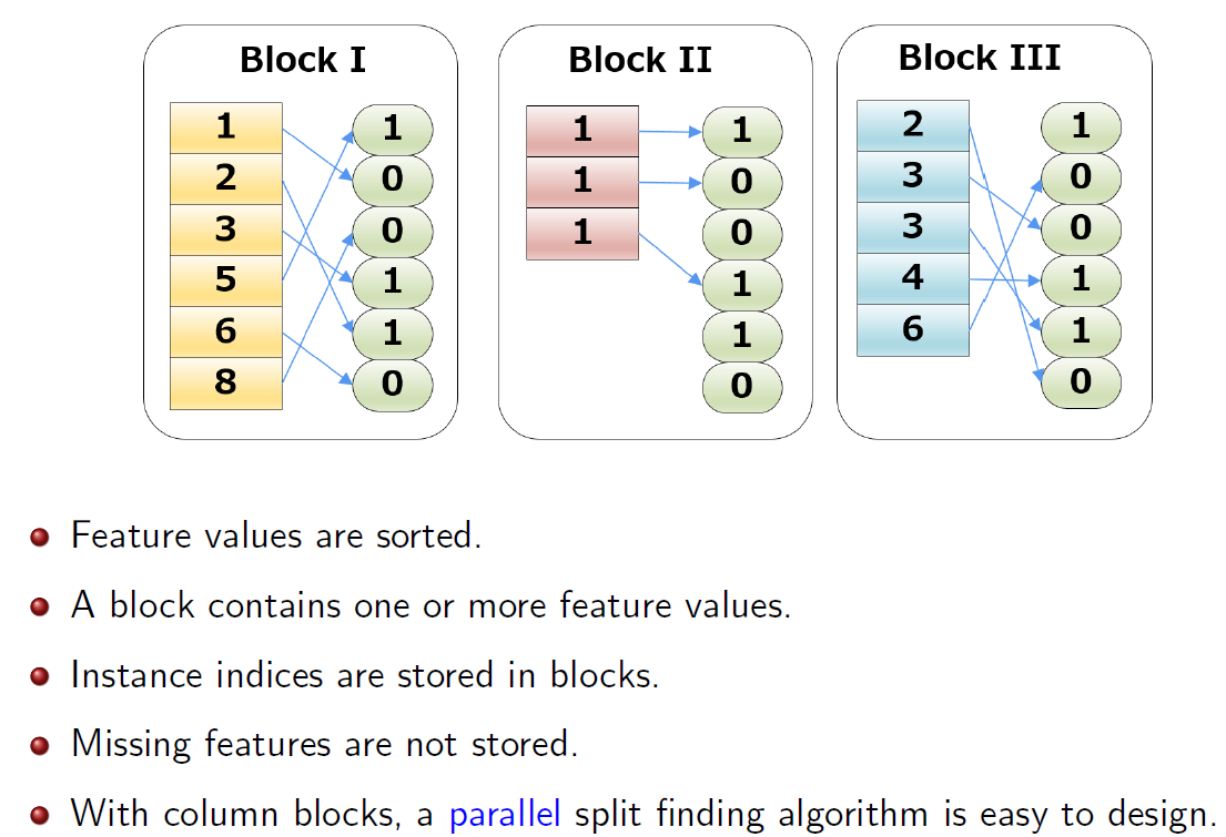
(1)Column Blocks and Parallelization
(2)Cache Aware Access
- A thread pre-fetches data from non-continuous memory into a continuous bu ffer.
- The main thread accumulates gradients statistics in the continuous buff er.
(3)System Tricks
- Block pre-fetching.
- Utilize multiple disks to parallelize disk operations.
- LZ4 compression(popular recent years for outstanding performance).
- Unrolling loops.
- OpenMP
7.程式碼走讀
這塊非常感謝楊軍老師的無私奉獻【4】
個人看程式碼用的是SourceInsight,由於xgboost有些檔案是cc字尾名,可以通過以下命令修改下(預設的識別不了)
find ./ -name "*.cc" | awk -F "." '{print $2}' | xargs -i -t mv ./{}.cc ./{}.cpp- 1
- 1
實際上,對XGBoost的原始碼進行走讀分析之後,能夠看到下面的主流程:
cli_main.cc:
main()
     -> CLIRunTask()
          -> CLITrain()
               -> DMatrix::Load()
               -> learner = Learner::Create()
               -> learner->Configure()
               -> learner->InitModel()
               -> for (i = 0; i < param.num_round; ++i)
                    -> learner->UpdateOneIter()
                    -> learner->Save()
learner.cc:
Create()
      -> new LearnerImpl()
Configure()
InitModel()
     -> LazyInitModel()
          -> obj_ = ObjFunction::Create()
               -> objective.cc
                    Create()
                         -> SoftmaxMultiClassObj(multiclass_obj.cc)/
                              LambdaRankObj(rank_obj.cc)/
                              RegLossObj(regression_obj.cc)/
                              PoissonRegression(regression_obj.cc)
          -> gbm_ = GradientBooster::Create()
               -> gbm.cc
                    Create()
                         -> GBTree(gbtree.cc)/
                              GBLinear(gblinear.cc)
          -> obj_->Configure()
          -> gbm_->Configure()
UpdateOneIter()
      -> PredictRaw()
      -> obj_->GetGradient()
      -> gbm_->DoBoost()

gbtree.cc:
Configure()
      -> for (up in updaters)
           -> up->Init()
DoBoost()
      -> BoostNewTrees()
           -> new_tree = new RegTree()
           -> for (up in updaters)
                -> up->Update(new_tree)

tree_updater.cc:
Create()
     -> ColMaker/DistColMaker(updater_colmaker.cc)/
        SketchMaker(updater_skmaker.cc)/
        TreeRefresher(updater_refresh.cc)/
        TreePruner(updater_prune.cc)/
        HistMaker/CQHistMaker/
                  GlobalProposalHistMaker/
                  QuantileHistMaker(updater_histmaker.cc)/
TreeSyncher(updater_sync.cc)- 1
- 2
- 3
- 4
- 5
- 6
- 7
- 8
- 9
- 10
- 11
- 12
- 13
- 14
- 15
- 16
- 17
- 18
- 19
- 20
- 21
- 22
- 23
- 24
- 25
- 26
- 27
- 28
- 29
- 30
- 31
- 32
- 33
- 34
- 35
- 36
- 37
- 38
- 39
- 40
- 41
- 42
- 43
- 44
- 45
- 46
- 47
- 48
- 49
- 50
- 51
- 52
- 53
- 54
- 55
- 56
- 1
- 2
- 3
- 4
- 5
- 6
- 7
- 8
- 9
- 10
- 11
- 12
- 13
- 14
- 15
- 16
- 17
- 18
- 19
- 20
- 21
- 22
- 23
- 24
- 25
- 26
- 27
- 28
- 29
- 30
- 31
- 32
- 33
- 34
- 35
- 36
- 37
- 38
- 39
- 40
- 41
- 42
- 43
- 44
- 45
- 46
- 47
- 48
- 49
- 50
- 51
- 52
- 53
- 54
- 55
- 56
從上面的程式碼主流程可以看到,在XGBoost的實現中,對演算法進行了模組化的拆解,幾個重要的部分分別是:
I. ObjFunction:對應於不同的Loss Function,可以完成一階和二階導數的計算。
II. GradientBooster:用於管理Boost方法生成的Model,注意,這裡的Booster Model既可以對應於線性Booster Model,也可以對應於Tree Booster Model。
III. Updater:用於建樹,根據具體的建樹策略不同,也會有多種Updater。比如,在XGBoost裡為了效能優化,既提供了單機多執行緒並行加速,也支援多機分散式加速。也就提供了若干種不同的並行建樹的updater實現,按並行策略的不同,包括:
I). inter-feature exact parallelism (特徵級精確並行)
II). inter-feature approximate parallelism(特徵級近似並行,基於特徵分bin計算,減少了列舉所有特徵分裂點的開銷)
III). intra-feature parallelism (特徵內並行)
此外,為了避免overfit,還提供了一個用於對樹進行剪枝的updater(TreePruner),以及一個用於在分散式場景下完成結點模型引數資訊通訊的updater(TreeSyncher),這樣設計,關於建樹的主要操作都可以通過Updater鏈的方式串接起來,比較一致乾淨,算是Decorator設計模式[4]的一種應用。
XGBoost的實現中,最重要的就是建樹環節,而建樹對應的程式碼中,最主要的也是Updater的實現。所以我們會以Updater的實現作為介紹的入手點。
以ColMaker(單機版的inter-feature parallelism,實現了精確建樹的策略)為例,其建樹操作大致如下:
updater_colmaker.cc:
ColMaker::Update()
     -> Builder builder;
     -> builder.Update()
          -> InitData()
          -> InitNewNode() // 為可用於split的樹結點(即葉子結點,初始情況下只有一個
                           // 葉結點,也就是根結點) 計算統計量,包括gain/weight等
          ->  for (depth = 0; depth < 樹的最大深度; ++depth)
               -> FindSplit()
                    -> for (each feature) // 通過OpenMP獲取
                                          // inter-feature parallelism
                         -> UpdateSolution()
                              -> EnumerateSplit()  // 每個執行執行緒處理一個特徵,
                                                   // 選出每個特徵的
                                                   // 最優split point
                              -> ParallelFindSplit()
                                   // 多個執行執行緒同時處理一個特徵,選出該特徵
                                   //的最優split point;
                                   // 在每個執行緒裡彙總各個執行緒內分配到的資料樣
                                   //本的統計量(grad/hess);
                                   // aggregate所有執行緒的樣本統計(grad/hess),
                                   //計算出每個執行緒分配到的樣本集合的邊界特徵值作為
                                   //split point的最優分割點;
                                   // 在每個執行緒分配到的樣本集合對應的特徵值集合進
                                   //行列舉作為split point,選出最優分割點
                         -> SyncBestSolution()
                               // 上面的UpdateSolution()/ParallelFindSplit()
                               //會為所有待擴充套件分割的葉結點找到特徵維度的最優split
                               //point,比如對於葉結點A,OpenMP執行緒1會找到特徵F1
                               //的最優split point,OpenMP執行緒2會找到特徵F2的最
                               //優split point,所以需要進行全域性sync,找到葉結點A
                               //的最優split point。
                         -> 為需要進行分割的葉結點建立孩子結點
               -> ResetPosition()
                      //根據上一步的分割動作,更新樣本到樹結點的對映關係
                      // Missing Value(i.e. default)和非Missing Value(i.e.
                      //non-default)分別處理
               -> UpdateQueueExpand()
                      // 將待擴充套件分割的葉子結點用於替換qexpand_,作為下一輪split的
                      //起始基礎
-> InitNewNode() // 為可用於split的樹結點計算統計量- 1
- 2
- 3
- 4
- 5
- 6
- 7
- 8
- 9
- 10
- 11
- 12
- 13
- 14
- 15
- 16
- 17
- 18
- 19
- 20
- 21
- 22
- 23
- 24
- 25
- 26
- 27
- 28
- 29
- 30
- 31
- 32
- 33
- 34
- 35
- 36
- 37
- 38
- 39
- 40
- 41
- 1
- 2
- 3
- 4
- 5
- 6
- 7
- 8
- 9
- 10
- 11
- 12
- 13
- 14
- 15
- 16
- 17
- 18
- 19
- 20
- 21
- 22
- 23
- 24
- 25
- 26
- 27
- 28
- 29
- 30
- 31
- 32
- 33
- 34
- 35
- 36
- 37
- 38
- 39
- 40
- 41
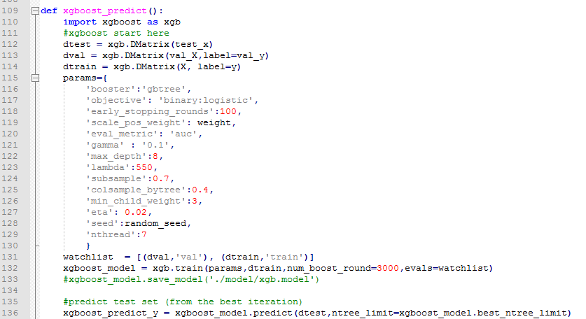
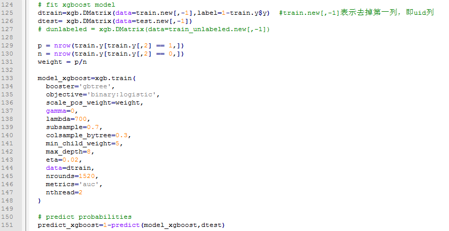
8.python、R對於xgboost的簡單使用
任務:二分類,存在樣本不均衡問題(scale_pos_weight可以一定程度上解讀此問題)
【R】
9.xgboost中比較重要的引數介紹
(1)objective [ default=reg:linear ] 定義學習任務及相應的學習目標,可選的目標函式如下:
- “reg:linear” –線性迴歸。
- “reg:logistic” –邏輯迴歸。
- “binary:logistic” –二分類的邏輯迴歸問題,輸出為概率。
- “binary:logitraw” –二分類的邏輯迴歸問題,輸出的結果為wTx。
- “count:poisson” –計數問題的poisson迴歸,輸出結果為poisson分佈。 在poisson迴歸中,max_delta_step的預設值為0.7。(used to safeguard optimization)
- “multi:softmax” –讓XGBoost採用softmax目標函式處理多分類問題,同時需要設定引數num_class(類別個數)
- “multi:softprob” –和softmax一樣,但是輸出的是ndata * nclass的向量,可以將該向量reshape成ndata行nclass列的矩陣。沒行資料表示樣本所屬於每個類別的概率。
- “rank:pairwise” –set XGBoost to do ranking task by minimizing the pairwise loss
(2)’eval_metric’ The choices are listed below,評估指標:
- “rmse”: root mean square error
- “logloss”: negative log-likelihood
- “error”: Binary classification error rate. It is calculated as #(wrong cases)/#(all cases). For the predictions, the evaluation will regard the instances with prediction value larger than 0.5 as positive instances, and the others as negative instances.
- “merror”: Multiclass classification error rate. It is calculated as #(wrong cases)/#(all cases).
- “mlogloss”: Multiclass logloss
- “auc”: Area under the curve for ranking evaluation.
- “ndcg”:Normalized Discounted Cumulative Gain
- “map”:Mean average precision
- “[email protected]”,”[email protected]”: n can be assigned as an integer to cut off the top positions in the lists for evaluation.
- “ndcg-“,”map-“,”[email protected]“,”[email protected]“: In XGBoost, NDCG and MAP will evaluate the score of a list without any positive samples as 1. By adding “-” in the evaluation metric XGBoost will evaluate these score as 0 to be consistent under some conditions.
(3)lambda [default=0] L2 正則的懲罰係數
(4)alpha [default=0] L1 正則的懲罰係數
(5)lambda_bias 在偏置上的L2正則。預設值為0(在L1上沒有偏置項的正則,因為L1時偏置不重要)
(6)eta [default=0.3]
為了防止過擬合,更新過程中用到的收縮步長。在每次提升計算之後,演算法會直接獲得新特徵的權重。 eta通過縮減特徵的權重使提升計算過程更加保守。預設值為0.3
取值範圍為:[0,1]
(7)max_depth [default=6] 數的最大深度。預設值為6 ,取值範圍為:[1,∞]
(8)min_child_weight [default=1]
孩子節點中最小的樣本權重和。如果一個葉子節點的樣本權重和小於min_child_weight則拆分過程結束。在現行迴歸模型中,這個引數是指建立每個模型所需要的最小樣本數。該成熟越大演算法越conservative
取值範圍為: [0,∞]
10.DART
核心思想就是將dropout引入XGBoost
示例程式碼
import xgboost as xgb
# read in data
dtrain = xgb.DMatrix('demo/data/agaricus.txt.train')
dtest = xgb.DMatrix('demo/data/agaricus.txt.test')
# specify parameters via map
param = {'booster': 'dart',
         'max_depth': 5, 'learning_rate': 0.1,
         'objective': 'binary:logistic', 'silent': True,
         'sample_type': 'uniform',
         'normalize_type': 'tree',
         'rate_drop': 0.1,
         'skip_drop': 0.5}
num_round = 50
bst = xgb.train(param, dtrain, num_round)
# make prediction
# ntree_limit must not be 0
preds = bst.predict(dtest, ntree_limit=num_round)- 1
- 2
- 3
- 4
- 5
- 6
- 7
- 8
- 9
- 10
- 11
- 12
- 13
- 14
- 15
- 16
- 17
- 1
- 2
- 3
- 4
- 5
- 6
- 7
- 8
- 9
- 10
- 11
- 12
- 13
- 14
- 15
- 16
- 17
更多細節可以閱讀參考文獻5
11.csr_matrix訓練XGBoost
當資料規模比較大、較多列比較稀疏時,可以使用csr_matrix訓練XGBoost模型,從而節約記憶體。
下面是Kaggle比賽中TalkingData開源的程式碼,可以學習一下,詳見參考文獻6。
import pandas as pd
import numpy as np
import seaborn as sns
import matplotlib.pyplot as plt
import os
from sklearn.preprocessing import LabelEncoder
from scipy.sparse import csr_matrix, hstack
import xgboost as xgb
from sklearn.cross_validation import StratifiedKFold
from sklearn.metrics import log_loss

datadir = '../input'
gatrain = pd.read_csv(os.path.join(datadir,'gender_age_train.csv'),
                      index_col='device_id')
gatest = pd.read_csv(os.path.join(datadir,'gender_age_test.csv'),
                     index_col = 'device_id')
phone = pd.read_csv(os.path.join(datadir,'phone_brand_device_model.csv'))
# Get rid of duplicate device ids in phone
phone = phone.drop_duplicates('device_id',keep='first').set_index('device_id')
events = pd.read_csv(os.path.join(datadir,'events.csv'),
                     parse_dates=['timestamp'], index_col='event_id')
appevents = pd.read_csv(os.path.join(datadir,'app_events.csv'),
                        usecols=['event_id','app_id','is_active'],
                        dtype={'is_active':bool})
applabels = pd.read_csv(os.path.join(datadir,'app_labels.csv'))

gatrain['trainrow'] = np.arange(gatrain.shape[0])
gatest['testrow'] = np.arange(gatest.shape[0])

brandencoder = LabelEncoder().fit(phone.phone_brand)
phone['brand'] = brandencoder.transform(phone['phone_brand'])
gatrain['brand'] = phone['brand']
gatest['brand'] = phone['brand']
Xtr_brand = csr_matrix((np.ones(gatrain.shape[0]),
                       (gatrain.trainrow, gatrain.brand)))
Xte_brand = csr_matrix((np.ones(gatest.shape[0]),
                       (gatest.testrow, gatest.brand)))
print('Brand features: train shape {}, test shape {}'.format(Xtr_brand.shape, Xte_brand.shape))

m = phone.phone_brand.str.cat(phone.device_model)
modelencoder = LabelEncoder().fit(m)
phone['model'] = modelencoder.transform(m)
gatrain['model'] = phone['model']
gatest['model'] = phone['model']
Xtr_model = csr_matrix((np.ones(gatrain.shape[0]),
                       (gatrain.trainrow, gatrain.model)))
Xte_model = csr_matrix((np.ones(gatest.shape[0]),
                       (gatest.testrow, gatest.model)))
print('Model features: train shape {}, test shape {}'.format(Xtr_model.shape, Xte_model.shape))

appencoder = LabelEncoder().fit(appevents.app_id)
appevents['app'] = appencoder.transform(appevents.app_id)
napps = len(appencoder.classes_)
deviceapps = (appevents.merge(events[['device_id']], how='left',left_on='event_id',right_index=True)
                       .groupby(['device_id','app'])['app'].agg(['size'])
                       .merge(gatrain[['trainrow']], how='left', left_index=True, right_index=True)
                       .merge(gatest[['testrow']], how='left', left_index=True, right_index=True)
                       .reset_index())

d = deviceapps.dropna(subset=['trainrow'])
Xtr_app = csr_matrix((np.ones(d.shape[0]), (d.trainrow, d.app)),
                      shape=(gatrain.shape[0],napps))
d = deviceapps.dropna(subset=['testrow'])
Xte_app = csr_matrix((np.ones(d.shape[0]), (d.testrow, d.app)),
                      shape=(gatest.shape[0],napps))
print('Apps data: train shape {}, test shape {}'.format(Xtr_app.shape, Xte_app.shape))

applabels = applabels.loc[applabels.app_id.isin(appevents.app_id.unique())]
applabels['app'] = appencoder.transform(applabels.app_id)
labelencoder = LabelEncoder().fit(applabels.label_id)
applabels['label'] = labelencoder.transform(applabels.label_id)
nlabels = len(labelencoder.classes_)

devicelabels = (deviceapps[['device_id','app']]
                .merge(applabels[['app','label']])
                .groupby(['device_id','label'])['app'].agg(['size'])
                .merge(gatrain[['trainrow']], how='left', left_index=True, right_index=True)
                .merge(gatest[['testrow']], how='left', left_index=True, right_index=True)
                .reset_index())
devicelabels.head()

d = devicelabels.dropna(subset=['trainrow'])
Xtr_label = csr_matrix((np.ones(d.shape[0]), (d.trainrow, d.label)),
                      shape=(gatrain.shape[0],nlabels))
d = devicelabels.dropna(subset=['testrow'])
Xte_label = csr_matrix((np.ones(d.shape[0]), (d.testrow, d.label)),
                      shape=(gatest.shape[0],nlabels))
print('Labels data: train shape {}, test shape {}'.format(Xtr_label.shape, Xte_label.shape))

Xtrain = hstack((Xtr_brand, Xtr_model, Xtr_app, Xtr_label), format='csr')
Xtest =  hstack((Xte_brand, Xte_model, Xte_app, Xte_label), format='csr')
print('All features: train shape {}, test shape {}'.format(Xtrain.shape, Xtest.shape))

targetencoder = LabelEncoder().fit(gatrain.group)
y = targetencoder.transform(gatrain.group)

########## XGBOOST #######