
Paper Reading: SSD
Outline
- 作者資訊:
- 二作Dragomir Anguelov,17年發表CVPR, CoRR兩篇二作,Stanford Univ. 研究領域Object detection
- 三作Dumitru Erhan, google brain senior,citation 15278
- 通訊作者Alex. Berg, UNC教授,一作導師,研究領域CV, citation 18407
- 關於Object detection
- - 輸入:圖片
- - 輸出:
- - location
- - 種類
- - 評價指標:
- - mAP
- - FPS(frame per second)
- 基於 CNNs 的 Object Detection 的已有工作有哪些?
- 人臉識別
- counting
- 衛星圖片物體檢測
- 本文的動機
- - 現在的benchmark(mAP):
- - 區域推薦 - 學習區域中的特徵 - 分類,如state of art Faster R-CNN
- - benchmark的缺點:
- - FPS = 7,太慢
- - 現在的benchmark(FPS then mAP):
- - 去除regional proposal的end-to-end NN,如state of art YOLO
- - benchmark的缺點:
- 速度的優化犧牲了準確率
- - 所以這篇文章產生了速度快的,準確率高的OD模型:SSD
- Related work
- (fig*2)
- 分為兩大類:sliding window 和 region proposal classification
- 在CNN之前:state of art 分別是DPM (Deformable(可變形) Part Model) 和 Selective Search
- 因為R-CNN的誕生,後者成為主流
- 首先運用selective search得到的region proposals的結果
- 把上面的結果尺寸變換放入AlexNet中
- 保留上面f7的輸出特徵再對針對每個類別訓練一個SVM的二分類器,label就是是否屬於該類別
測試階段最後再通過svm的分類器對之前的proposal進行訓練,得到每個類別修正之後的bounding box
- 也就是把卷積網路的輸出做svm的分類,結合了Selective search 和 conv network based post-classification
- R-CNN = Selective search + AlexNet + SVM
- R-CNN的第一次升級:speed up post-classification, 因為post-classification這個過程十分耗時消耗記憶體,因為他要將幾千個image的裁剪結果進行分類。
- SPPnet:
- pros: 發明了spatial pyramid pooling layer, 對區域的大小和規模更加robust
- 並且讓classification layers 複用之前在不同的解析度的feature map上學習到的特徵。
- SPP layer(ROI pooling layer是SPP layer的特例:相當於只有一層的空間金字塔):把不同尺寸的featrue map上的框框的pooling為相同的,固定大小的feature。
- 框框從不同到相同的過程:做不同level的pooling,然後把他們pooling的結果串在一起!
- Fast R-CNN:
- 運用了SPP layer,去掉SVM部分,把AlexNet最後一層的輸出連結到ROI pooling layer上(SPP的特例!),讓他尺寸固定。
- 再把這個固定size的輸出分叉,一個去softmax,一個去bbox的迴歸。
- loss fun不再是分開的,loss = bounding box regression + conf, 實現了end-to-end tuning
Fast R-CNN = Selective search + AlexNet + ROI pooling + 分叉實現兩個pred,loss結合兩個loss
- R-CNN系列的第二次升級:改善regional proposal:using deep neural networks
- MultiBox:
- Selective search的缺點:用的是low level的feature
- 所以用一個separate的神經網路替代
- pros:regional proposal 準確率更高
- cons: 太複雜了,兩個網路要結合在一起訓練比較複雜。
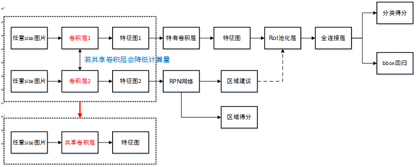
- Faster R-CNN
- 利用了RPN:region proposal network
- pool了mid-level feature
- 讓最終的分類過程不那麼expensive
- RPN中包含了anchor box(fixed)的概念,很想ssd的default box
- Faster R-CNN = RPN + Fast R-CNN(原來是ss)
- cons: RPN+Fast R-CNN太複雜了,要分別預訓練
- RPN中的anchor box是為了提取特徵(pool feature),生成feature map,再把feature map放到RPN裡面得到每個fixed anchor是否有物體,然後把結果放到classification layer裡面,找出他的class和bounding regression。
- 但是SSD是通過default box同時預測出這一個box中所有種類的box的confidence。
- 另一個系列:sliding window和ssd是一個系列的,
- 去掉了proposal的階段!
- 直接預測位置+不同種類的object的confidence
- Overfeat:
- 把sliding window的過程換成了conv layer,最後的輸出是2*2*4的話代表左上右上左下右下分別是四個class的confidence
- 缺點:loc的精確度太低了
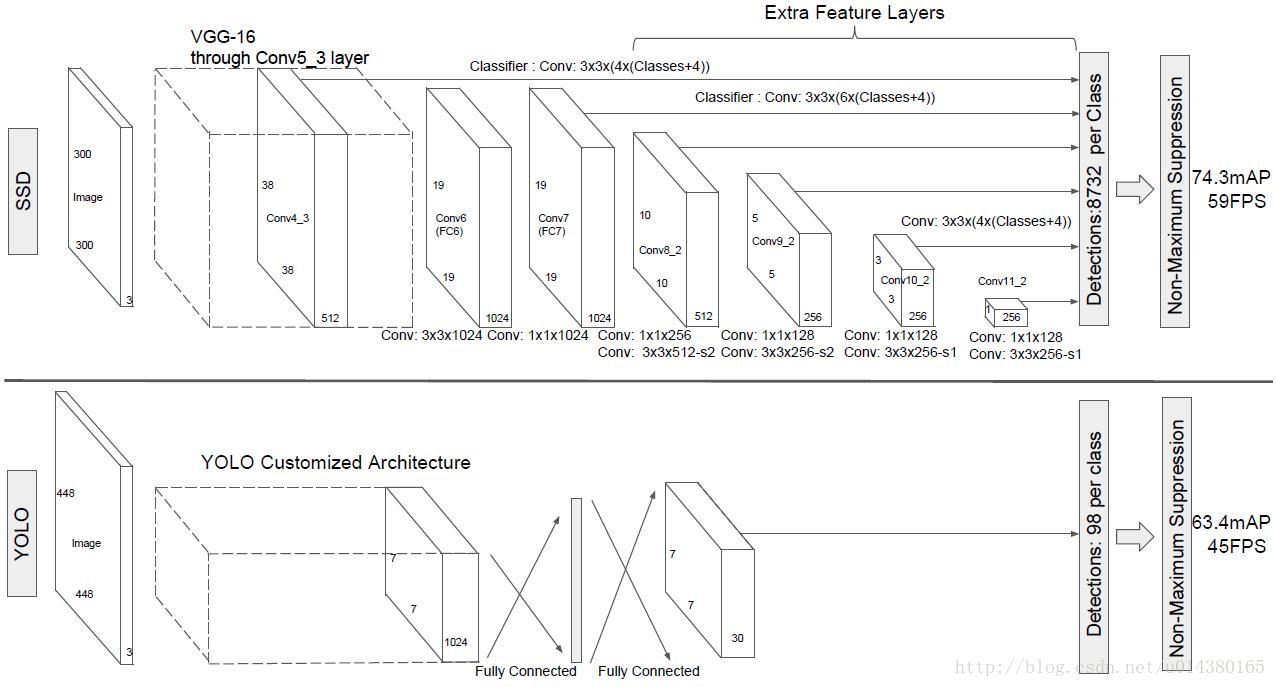
- Yolo:
- 使用top most feature map(就是lower feature map,沒有經過conv的size收縮)同時提取bbox & all class conf
- 問題:沒有考慮anchor box的不同的aspect ratio
- SSD vs Overfeat:
- Oerfeat只用了topmost feature map
- Overfeat沒有使用multi aspect ratio的default box(retio=1)
- SSD s YOLO:
- Yolo只用了topmost feature map
- Yolo沒有使用multi aspect ratio的default box
YOLO:each grid cell only predicts two boxes,不像ssd那麼多類而且還可以有不同的ratio
YOLO:can only have one class for one box, 但是SSD的一個default box可以和任何一個IoU > 0.5 的gt match
YOLO認為:
- DPM(Deformable parts models)太慢太不準
- R-CNN這個pipeline太慢太複雜,因為要分別tune precisely
- SS給出的proposal太多了
- Faster R-CNN:
- 比R-CNN更快
- 比R-CNN更準
- 但還是太慢了 不能real time
- Deep multibox:
- Multibox僅僅是ss的替代品
- 它只是大figure裡面的小pipe,不完整
- 它雖然不用ss但是還用further image patch classification呀
- Over feat:
- 是sliding window神一樣的改進
- 但還是disjoined system
- 只優化了定位,沒有優化detection performance
- 只能看到區域性資訊,浪費了global info
- 所以需要後期處理來deal with相連的detection
- MultiGrasp
- grasp detection比object detection簡單多了
- 只需要找到圖裡面的一個object,不需要分來,loc,估計大小,估計boundary
- 總之功能太弱了
- 效能分析
- (fig)
- - why high speed?
- - 去掉了Regional proposal, feature resampling,subsequent pixel的階段(as Overfeat和YOLO)。
- - 但是真的能說明更快嗎?
- - SSD:300*300
- - YOLO:448*448 (faster than YOLO cuz SSD512 performs faster)
- - Faster R-CNN:600*1000 (false!)
- - why high acc?
- - small conv filter to predict class & bounding box with:
- - feature maps from different layer - have diff scales of boxes
- - diff aspect ratio - have diff shapes of boxes
- - 對於解析度低的圖片(圖片更小)有更高的準確率和速度
- - 所以可能準確性更高了,但是並不能證明速度!
- 核心特徵:
- - 讓輸出的空間離散+濃密的box分佈(從濃密到稀疏)
- - multi scale feature map prediction
- - 從多個不同解析度的feature map上進行不同class的不同位置、不同scale(也就是每個box對應原圖的大小)、不同的confidence的default box的class和bounding box偏移的結果。
- - 和Faster R-CNN的anchor box的區別
- - Faster & Overfeatr:只在大小固定的feature map上形成一次bounding box
- - SSD:在不同scale的feature map上分別形成default box
- - why multi feature maps?
- - (box num fig)
- - suitable for multi-size objects (receptive field size) 仿照了從不同尺寸處理照片
- - 共享引數,用一個kernel conv所有的照片的同feature map的所有position
- - why multi boxes instead of 1 box per location like Overfeat
- - more boxes, more densely the space would be separated
- - more box, higher accuracy of location: (cat dog fig)
- - a single network
- - 沒有以下操作:
- - Regional proposal(R-CNN系列)
- - feature resampling
- - subsequent pixel(後面兩項指的是先有了regional proposal,再從這個region學習新的特徵/子特徵)
- - easy to train
- - straightforward
- - 沒有以下操作:
- 模型描述:
- (fig.2)
- - Inference階段
- - Input Image
- - on different feature maps:get the box and class applying small conv kernels (3*3-s1, pad=1)
- subinput: the conv layer (like conv4_3 result), shape = (h, w, 512)
- suboutput1: the confidence for each class: shape = (h, w, k*num_class), where k is the box num on each position
- suboutput1: the loc for each class: shape = (h, w, k*4)
- - continue conv steps
- - use nms on each class (before which: threshold selection) cuz so much boxes. IoU > 0.45 per class 中nms,最後keep top200個box。比較耗時
- - get final boxes
- - calculate mAP
- 每一步的輸入輸出都是什麼
SSD300, VOC2007
| Input layer | 300,300,3 | VGG16 till conv4_3 | 38,38,512(conv4_3) | ||
| conv4_3 | 38,38,512 | VGG16 conv4_3 till POOL5(3*3-s1, pad=1) | 19,19,512(pool5) | conv 3*3*(4*class) conv 3*3*(4*4) | 38*38*(4*class) 38*38*(4*4) |
| fc6(conv6) | 19,19,512 | conv 3*3*1024, same conv 1*1*1024 | 19,19,1024(fc7) | ||
| fc7(conv7) | 19,19,1024 | conv 1*1*256 conv 3*3*512-s2, p=1 | 10,10,512(conv8_2) | conv 3*3*(6*class) conv 3*3*(6*4) | 19*19*(6*class) 19*19*(6*4) |
| conv8_2 | 10,10,512 | conv 1*1*126 conv 3*3*256-s2 | 5,5,256(conv9_2) | conv 3*3*(6*class) conv 3*3*(6*4) | 10*10*(6*class) 10*10*(6*4) |
| conv9_2 | 5,5,256 | conv 1*1*126 conv 3*3*256-s1 | 3,3,256(conv10_2) | conv 3*3*(6*class) conv 3*3*(6*4) | 5*5*(6*class) 5*5*(6*4) |
| conv10_2 | 3,3,256 | conv 1*1*126 conv 3*3*256-s1 | 1,1,256(conv11_2) | conv 3*3*(4*class) conv 3*3*(4*4) | 3*3*(4*class) 3*3*(4*4) |
| conv11_2 | 1,1,256 | conv 3*3*(4*class) conv 3*3*(4*4) | 1*1*(6*class) 1*1*(4*4) |
Total boxes: 38*38*4+19*19*6+10*10*6+5*5*6+3*3*4+1*1*4=8732 * class
網路主線時間複雜度:
網路conv detector hierarchy分支的時間複雜度:
- O(sum(m*n, 3^2, C_featureMapChannel, (#boxPerPosition)(#class+4))
上面二者求和即可
- - Training階段
- - labeling: matching strategy (which boxes are Pos)
- - match gt to box with highest IoU
- - match gt to any box with IoU > 0.5
- - Aim: simplify training,更方便收斂
- Pos result:
- 上面有gt相匹配的db
- TP:
- 在上面Pos result之中
- IoU > Threshold
- Class is corret
- FP:
- 在上面的Pos result之中
- 不是TP的box
- - how to choose default box
- - 讓scale的分佈在每一個feature map上更加均勻,線性遞增
- - (公式)
- - loss func: SmoothL1(box param) + Softmax(class prob)
- - why smooth: less sensitive to outliers, small dist -> smaller smooth
- - loc loss is only about Pos boxes
- - class loss: all Pos + some Neg
- - hard negative mining
- - 為了減少FP,讓Neg:pos最大=3:1
- - 好處:降低FP,訓練更快
- - data aug
- - 方式:
- - 水平翻轉
- - 隨機裁剪,顏色,扭曲
- - 隨機擴張(zoom out,擴張補灰色)
- - VOC07: 8.8%mAP
- - Faster R-CNN不會因此更精準的原因:有一個ROI pooling的過程讓圖片縮放成一個size,所以對大小十分robust
- - 對小物體效果好
- - 但是training需要更長時間的迭代
- - 方式:
- - 需要考慮的引數
- - tiling of db: position & scale,能否和receptive field更好的排列,分佈更均勻
- - labeling: matching strategy (which boxes are Pos)
- 實驗
- - 資料集:
- - PASCAL VOC資料集, 包括20個目標超過11,000影象,超過27,000目標bounding box。其資料集影象質量好,標註完備,非常適合用來測試演算法效能.
- 特點:資料量少,質量好 + 資料種類少(20)
- - COCO資料集有超過 200,000 張圖片,80種物體類別. 所有的物體例項都用詳細的分割mask進行了標註,共標註了超過 500,000 個物體實體
- 特點:object較小,資料量大,資料種類多(80)
- - ImageNet資料下的ILSVRC檢測資料集分為三個集:train(395,918),val(20,121)和test(40,152)
- 特點:資料量大 + 資料種類很多(200)
- - val1用來訓練
- - val2用來測試,其中200個類的類別分佈都比較均衡(val1中和val2中的類大體重合)
- - PASCAL VOC資料集, 包括20個目標超過11,000影象,超過27,000目標bounding box。其資料集影象質量好,標註完備,非常適合用來測試演算法效能.
- - 引數
- - 10-3 staging change
- - 0.9 momentum
- - 0.0005 weight decay - overfitting
- - 實驗1: PASCAL VOC2007
- - info
- - test:4952 (small)
- - SSD300: 6 maps,SSD512: 7 maps
- - Xavier init
- - conv4_3 = 0.1
- - 為什麼conv4_3用了L2 norm來調整scale:lower feature差異較大
- - lr staging change比較快
- - SSD512:
- - 添加了conv12_2上的conv detector
- - min = 0.15, conv4_3 = 0.07
- - 為什麼scale的最小值要縮小:
- - 為了讓不同的feature map對應的不同的scale更加均勻,對小的物體的檢測效果更好。層變多了,如果不改scale,可能scale會集中在0.2-0.9之間,過於密集
- - 得到更多box
- - result:
- 資料集越大mAP越高,從07+12開始超越R-CNN系列
- - 分析(FIg4)
- - loc更精準,因為有了更精準的box
- - simi class難區分,因為兩個不同的class可能有很相近的location,比如貓狗那張圖片,中間的box會不知道是which one(圖貓狗)
- - 對大小敏感,小物體很差
- - lower layer, higher 已經不存在了
- - lower layer, lower feature, 不好classification
- - lower layer感受野太小,感受不到全域性的feature,只能提取到local
- - 對不同形狀因為有不同長款比所以效能很好(放圖Fig4)
- - 優化問題
- - 更多ratio更好:
- - 問題,沒有保證#box數量不變吧
- - atrous is faster:
- - 問題,變數太多了吧:
- - 2*2 -s2 vs 3*3-s1,
- - atrous vs no-atrous
- - conv5_3 pred vs no-conv5_3 pred
- - multi-scale feature map 更好
- - 一層一層減少,保證bounding box數量不變,mAP下降
- - 關於是否應當去掉邊界的box:
- - 如果使用了高層featuremap,去掉會十分影響,因為pruned a lot boxes
- - 如果沒有使用高層,去掉影響不大
- - 更多ratio更好:
- - info
- - 實驗2:PASCAL VOC2012
- - 資料:
- - trainnval = 12trainval+07trainval + 07test
- - test = 12test
- - 引數:iter更多
- - result:mAP碾壓
- - 資料:
- - 實驗3:COCO
- - (table5)
- - 資料:
- - 類別非常多(80)
- - object small
- - training:trainval35k
- - test:test-dev2015
- - 引數:
- - IoU Pos threshold:[email protected]後面的引數的平均值
- - iter更多
- - s_min=0.15(512=0.1);conv4_3=0.07(512=0.04)為了檢測小的物體,讓最小的scale更小
- - result
- - SSD300總體來說挺差的,除了在大物體檢測的APAR超過了之前的(100個點)要比ION和faster差。
- - Faster的小物體檢測特別好。
- - SSD512還是碾壓的
- - 關於為什麼@0.75似乎比@0.5還要好
- - 位置準確性:ssd performs better,(loss of loc控制的好)說明了多scale多box的好處:denser
- - 實驗4:ILSVRC的簡單訓練:
- - 資料
- - ILSVRC2013檢測資料集分為三個集:train(395,918),val(20,121)和test(40,152)
- - val1用來訓練
- - val2用來測試,其中200個類的類別分佈都比較均衡(val1中和val2中的類大體重合)
- - 模型:
- - SSD300:43.4mAP
- - 引數
- - lr變化慢,iter非常長
- - 資料
- Future work
- - Base net speed up
- - db tiling method
- 總結
- pros
- 執行速度可以和YOLO媲美,檢測精度可以和Faster RCNN媲美。
- 因為從輸入到輸出是一個整體,不像RCNN是先有proposal再進行訓練,所以更直觀,更easy to train
- 對於解析度低的資料也有很好的表現
- cons
- 需要人工設定prior box的min_size,max_size和aspect_ratio值。網路中prior box的基礎大小和形狀不能直接通過學習獲得,而是需要手工設定。而網路中每一層feature使用的prior box大小和形狀恰好都不一樣,導致除錯過程非常依賴經驗。
- tiling方案
- 雖然採用了pyramdial feature hierarchy的思路,但是對小目標的recall依然一般,並沒有達到碾壓Faster RCNN的級別。由於SSD使用conv4_3低階feature去檢測小目標,而低階特徵卷積層數少,存在特徵提取不充分的問題。
- data aug
- 多層的feature沒有共享資訊,可以考慮FPN結合了每一個feature map的global特徵
- 浪費時間主要在vgg16上
- basenet提速
- 最大的FP在於similar class,相鄰的class還是不好檢測,因為中間的default box(包含了兩個類)會不知道自己被放到哪個class裡面比較好
- 提高解析度,使用更加密集的db
- 需要人工設定prior box的min_size,max_size和aspect_ratio值。網路中prior box的基礎大小和形狀不能直接通過學習獲得,而是需要手工設定。而網路中每一層feature使用的prior box大小和形狀恰好都不一樣,導致除錯過程非常依賴經驗。
- 問題
- 對比方式:不一定更快
- atrous更好的證明
- more aspect ratio更好的證明
ssd/ssd_pascal.py
- benchmark基本資訊
列舉所有模型、訓練相關的引數,定性討論每個引數對效能的影響
input wieight & heightuse boundary - 如果使用higher feature map(with hight scale), 效能變差,如果不使用higher feature, 效能沒什麼大變化batch - 有助於FPS,size=8對mAP沒有影響data aug- 裁剪min_jaccard_overlap: 0.1 0.3 0.5 0.7 0.9 (1.0) 有利於識別小物體- num of each min_jaccard_overlap:50- aug scale [0.1-1] # 隨機裁剪,有利於zoom in功效- aspect ration [0.5-2] #裁剪的aspect ratio,有利於不同形狀物體識別- distort- expandprob:0.5,max_expand_ratio:4.0,zoom out,生成更多的小物體use batchnorm = False,iftrue, should use batch normforall newly added layers因為還沒有測試有batchnorm的performance如果有BN,base_lr 0.0004,else: 0.00004base_lr 0.00004weight_decay = 0.0005 # penalty防止過擬合lr_policy = multistepstepvalue = 12w,10w,8w # 資料集變大or資料尺寸變大,step也要變大momentum = 0.9 # 優化SGD方向type:SGD# multibox paramsn_classes: 21bg_lable = 0ignore cross boundary bbox =falsehard negative mining: neg_pos_ratio=3 # 防止過分關注FPmining type: max_negativeshare location:truetrain on diff dt:true?????loc_weight = (neg_pos_ratio + 1.) / 4.如果neg更多,loc的比重應該越大,因為loc裡面只有Pos,而conf=Pos + Neg,要多關注TPmultibox_loss_param = {'loc_loss_type': P.MultiBoxLoss.SMOOTH_L1, # less sensitive to outliers'conf_loss_type': P.MultiBoxLoss.SOFTMAX,'loc_weight': loc_weight,'num_classes': num_classes,'share_location': share_location,'match_type': P.MultiBoxLoss.PER_PREDICTION,'overlap_threshold': 0.5, # 大於0.5算作匹配,越大匹配的db越少,越不利於訓練'use_prior_for_matching': True, # ???'background_label_id': background_label_id,'use_difficult_gt': train_on_diff_gt,'mining_type': mining_type,'neg_pos_ratio': neg_pos_ratio,'neg_overlap': 0.5, # ???'code_type': code_type,'ignore_cross_boundary_bbox': ignore_cross_boundary_bbox,}loss_param = {'normalization': normalization_mode,}# feature maps# conv4_3 ==> 38 x 38# fc7 ==> 19 x 19# conv6_2 ==> 10 x 10# conv7_2 ==> 5 x 5# conv8_2 ==> 3 x 3# conv9_2 ==> 1 x 1mbox_source_layers = ['conv4_3','fc7','conv6_2','conv7_2','conv8_2','conv9_2']# in percent %min_ratio = 20max_ratio = 90step =int(math.floor((max_ratio - min_ratio) / (len(mbox_source_layers) - 2)))min_sizes = []max_sizes = []forratio in xrange(min_ratio, max_ratio + 1, step):min_sizes.append(min_dim * ratio / 100.)max_sizes.append(min_dim * (ratio + step) / 100.)min_sizes = [min_dim * 10 / 100.] + min_sizesmax_sizes = [min_dim * 20 / 100.] + max_sizes'''[30.0, 60.0, 111.0, 162.0, 213.0, 264.0][60.0, 111.0, 162.0, 213.0, 264.0, 315.0]'''steps = [8, 16, 32, 64, 100, 300] # receptive fieldaspect_ratios = [[2], [2, 3], [2, 3], [2, 3], [2], [2]]# L2 normalize conv4_3. # lwoer features have higher varnormalizations = [20, -1, -1, -1, -1, -1]# variance used to encode/decode prior bboxes.ifcode_type == P.PriorBox.CENTER_SIZE:prior_variance = [0.1, 0.1, 0.2, 0.2]else:prior_variance = [0.1]flip = Trueclip = False# Roughly there are 2000 prior bboxes per image.# TODO(weiliu89): Estimate the exact # of priors.base_lr *= 2000.# Evaluate on whole test set.num_test_image = 4952test_batch_size = 8# Ideally test_batch_size should be divisible by num_test_image,# otherwise mAP will be slightly off the true value.test_iter =int(math.ceil(float(num_test_image) / test_batch_size))solver_param = {# Train parameters'base_lr': base_lr,'weight_decay': 0.0005,'lr_policy':"multistep",'stepvalue': [80000, 100000, 120000],'gamma': 0.1,'momentum': 0.9,'iter_size': iter_size,'max_iter': 120000,'snapshot': 80000,'display': 10,'average_loss': 10,'type':"SGD",'solver_mode': solver_mode,'device_id': device_id,'debug_info': False,'snapshot_after_train': True,# Test parameters'test_iter': [test_iter],'test_interval': 10000,'eval_type':"detection",'ap_version':"11point",'test_initialization': False,}# parameters for generating detection output.det_out_param = {'num_classes': num_classes,'share_location': share_location,'background_label_id': background_label_id,'nms_param': {'nms_threshold': 0.45,'top_k': 400}, # 最終經過nms後保留400個box,overlap > 0.45的進行nms'save_output_param': {'output_directory': output_result_dir,'output_name_pix':"comp4_det_test_",'output_format':"VOC",'label_map_file': label_map_file,'name_size_file': name_size_file,'num_test_image': num_test_image,},'keep_top_k': 200, # 最終經過nms後保留400個box'confidence_threshold': 0.01,'code_type': code_type,}# parameters for evaluating detection results.det_eval_param = {'num_classes': num_classes,'background_label_id': background_label_id,'overlap_threshold': 0.5,'evaluate_difficult_gt': False,'name_size_file': name_size_file,}eReference:
- ECCV Slides
沒有想到的點/意識到的問題
- 關於Presentation
- 最好直接用原文的英文單詞不要自己翻譯。
- 記得列出參考文獻。
- 引數列表應該分類更清晰一些,如training, inference等。
- 關於演算法
- 正例和負例沒有理解對(vs TP FP)
- 關於matching strategy 是否會導致一隻大狗被檢測成了兩隻小狗的問題?
- 其實不是matching strategy的問題,而是正常的OD演算法都存在這個問題,因為幾乎任何的OD演算法都可能在一個gt上產生多個inference box。
- 思考:為什麼要有這樣的matching strategy:
- 否則可能有更多gt沒有一個inference box能match上他的問題。有更多的matching bbox可以增加正例,並讓更多的gt被檢測到(不被遺漏)。
- 否則可能有更多gt沒有一個inference box能match上他的問題。有更多的matching bbox可以增加正例,並讓更多的gt被檢測到(不被遺漏)。
- 關於實驗
- AR的實驗是否合理?
- 關於ar的實驗,之前認為bbox的數量沒有保持不變所以有問題,但是實際上這兩個屬性出發點是一樣的,都是為了更好地fit物體,所以上面的ref的slides裡面並沒有說AR而是說了box更多更好。
因為更多的tiling about box就是通過增加AR實現的。所以作者並沒有區別更多box和更多aspect ratio,這兩個概念在paper裡是等同的。
- 關於ar的實驗,之前認為bbox的數量沒有保持不變所以有問題,但是實際上這兩個屬性出發點是一樣的,都是為了更好地fit物體,所以上面的ref的slides裡面並沒有說AR而是說了box更多更好。
- faster R-CNN是否具有尺寸不變性
- 文中只是提及了更好的位置不變性(robust to object translation & data augmentation可能less important)。
- AR的實驗是否合理?
- 最後提到的比較難解的問題
- 哪個模型的效能會更好???(給出一個整體評價)在實際中應當如何選擇?(TODO)
- e.g.對於自行車,使用1/2和1/1的AR的box,會有什麼區別?
- 理解:形狀一致一個gt會匹配更多的bbox,所以會出現更多的正例,對training收斂有幫助。
可以假設object的AR是8:1的時候用了1:8的AR的default box,會幾乎不會有bbox可以匹配到gt上面,所以在訓練時這樣的gt就會被忽略掉,最終模型可能檢測這樣的gt的mAP非常低。
- 理解:形狀一致一個gt會匹配更多的bbox,所以會出現更多的正例,對training收斂有幫助。
- 在matching階段用了AR,在計算loss階段沒有使用AR(bug,比如產生box的堆疊),會有什麼結果?
- matching階段一個gt匹配了很多的box
相當於在同一個地方用了k個一樣的3*3的卷積核,其實是沒有區別的。因為在conv detect階段是不會區分不同ar的(假設計算Loss偏移量L_loc的時候使用了ar的bounding box)。只是在計算loss階段需要了正例負例的資訊,而這些資訊是從matching階段產生的。 - 如果在通過偏移量計算loss時也忘記了AR,那麼這個bug就必須fix掉了...因為inference的結果是不準確的。
- matching階段一個gt匹配了很多的box
- 哪個模型的效能會更好???(給出一個整體評價)在實際中應當如何選擇?(TODO)
其他
- mAP計算
- SSD和Faster R-CNN效能對比,如果SSD的input size變為同Faster R-CNN效能會如何變化
- Multi feature map上的scale如何選擇(open problem)
- Hard Negtive Mining的目的
- ....
相關推薦
Paper Reading: SSD
Outline- 作者資訊:二作Dragomir Anguelov,17年發表CVPR, CoRR兩篇二作,Stanford Univ. 研究領域Object detection三作Dumitru Erhan, google brain senior,citation 152
【Paper Reading】Bayesian Face Sketch Synthesis
bayesian .com ext tar mod images problem str targe Contribution: 1) Systematic interpretation to existing face sketch synthesis methods.
Paper Reading: Recombinator Networks: Learning Coarse-to-Fine FeatureAggregation
大小 destroy normal png post 結構化 del AC ear Github 源碼: https://github.com/SinaHonari/RCN convnet 存在的問題: max-pooling: for tasks requiring p
【Paper Reading】Learning while Reading
協作 每一個 info ++ 平時 arr 向上 移除 否則 Learning while Reading 不限於具體的書,只限於知識的寬度 這個系列集合了一周所學所看的精華,它們往往來自不只一本書 我們之所以將自然界分類,組織成各種概念,並按其分類,
paper reading----Xception: Deep Learning with Depthwise Separable Convolutions
module 之間 pap AD lin reg arch dual pooling 背景以及問題描述: Inception-style models的基本單元是Inception module。Inception model是Inception mod
Paper Reading - Convolutional Image Captioning ( CVPR 2018 )
useful rom ets ict inno entropy indexing com rtu Innovations: The authors develop a convolutional ( CNN-based ) image captioning method
paper reading:gaze tracking
tps sin nbsp papers https ont pen pdf aid https://www.cv-foundation.org/openaccess/content_cvpr_2016/papers/Krafka_Eye_Tracking_for_CVPR_
Paper Reading - Attention Is All You Need ( NIPS 2017 )
int tput represent enc perf task desc compute .com Link of the Paper: https://arxiv.org/abs/1706.03762 Motivation: The inherently sequen
paper reading: TP-GAN
Beyond Face Rotation: Global and Local Perception GAN for Photorealistic and Original Paper: TP-GAN Abstract TP-GAN simultaneously pe
Paper Reading: Pose-Aware Face Recognition in the wild
Pose-Aware Face Recognition in the wild (CVPR 2016) paper link: https://www.cv-foundation.org/openaccess/content_cvpr_2016/papers/Masi_Pose-Awar
[Paper Reading] A QoE-based Sender Bit Rate Adaptation Scheme for Real-time Video Transmission
A QoE-based Sender Bit Rate Adaptation Scheme for Real-time Video Transmission in Wireless Networks 發表 這篇文章發表於CISP2013,作者是南郵的Chao Qian。 概述
Paper reading:BodyNet: Volumetric Inference of 3D Human Body Shapes
標題:BodyNet: Volumetric Inference of 3D Human Body Shapes 作者:Gul Varol, Duygu Ceylan Bryan Russell Jimei Yang Ersin Yumer,z Ivan La
Paper Reading 之(1)AlexNet
Paper Krizhevsky, Alex, Ilya Sutskever, and Geoffrey E. Hinton. “Imagenet classification with deep co
Paper Reading——LEMNA:Explaining Deep Learning based Security Applications
bsp paper mat ant function using for arr class Motivation: The lack of transparency of the deep learning models creates key barriers to
[paper reading] C-MIL: Continuation Multiple Instance Learning for Weakly Supervised Object Detection CVPR2019
ppi ges cores sets spatial 完整 with rop ima MIL陷入局部最優,檢測到局部,無法完整的檢測到物體。將instance劃分為空間相關和類別相關的子集。在這些子集中定義一系列平滑的損失近似代替原損失函數,優化這些平滑損失。 C-MIL
SIGIR2018 Paper Abstract Reading Notes (1)
single for 很大的 領域 recent 個性化推薦 ranking 代理 公開 1.A Click Sequence Model for Web Search(日誌分析) 更好的理解用戶行為對於推動信息檢索系統來說是非常重要的。已有的研究工作僅僅關註於建模和預測一
Tools for reading paper[astro]
astrobits 上的一篇文章,挺好的,要是去年先看了就好了 https://astrobites.org/2017/12/19/tools-for-reading-papers-part-1/ https://astrobites.org/2018/03/09/tools-for-rea
Reading Level Assessment Using Support Vector Machines and Statistical Language Models-paper
Authors: Sarah E. Schwarm University of Washington, Seattle, WAMari Ostendorf University of Washington, Seattle, WAPublished in: ACLtime:June 25 - 30, 2005
SAS SATA SSD基本介紹
異步io 半導體 也有 不存在 線纜 讀寫性能 解決 異步 流動 SATA硬盤采用新的設計結構,數據傳輸快,節省空間,相對於IDE硬盤具有很多優勢: 1 .SATA硬盤比IDE硬盤傳輸速度高。目前SATA可以提供150MB/s的高峰傳輸速率。今後將達到300 MB/s和
Caffe上用SSD訓練和測試自己的數據
輸出 makefile b數 text play cal 上下 lba san 學習caffe第一天,用SSD上上手。 我的根目錄$caffe_root為/home/gpu/ljy/caffe 一、運行SSD示例代碼 1.到https://github.com