
RandomForest:隨機森林
隨機森林:RF
隨機森林是一種一決策樹為基學習器的Bagging演算法,但是不同之處在於RF決策樹的訓練過程中還加入了隨機屬性選擇(特徵上的子取樣)
- 傳統的決策樹在選擇劃分的屬性時,會選擇最優屬性
- RF
- 首先,從該節點的屬性中損及選擇出K個屬性組成一個隨機子集(類也就是Bagging中的Random Subspaces,一般通常K=log2(n))
- 然後再從這個子集中選擇一個最右子集進行劃分
引數
使用這些方法時要調整的引數主要是 n_estimators 和 max_features。 前者(n_estimators)是森林裡樹的數量,通常數量越大,效果越好,但是計算時間也會隨之增加。 此外要注意,當樹的數量超過一個臨界值之後,演算法的效果並不會很顯著地變好。 後者(max_features
max_features = n_features, 分類問題使用max_features = sqrt(n_features (其中 n_features 是特徵的個數)是比較好的預設值。max_depth = None和 min_samples_split = 2 結合通常會有不錯的效果(即生成完全的樹)。 請記住,這些(預設)值通常不是最佳的,同時還可能消耗大量的記憶體,最佳引數值應由交叉驗證獲得。 另外,請注意,在隨機森林中,預設使用自助取樣法(bootstrap = True), 然而 extra-trees 的預設策略是使用整個資料集(bootstrap = False)。 當使用自助取樣法方法抽樣時,泛化精度是可以通過剩餘的或者袋外的樣本來估算的,設定 oob_score = True提示:
預設引數下模型複雜度是:O(M*N*log(N)) , 其中 M 是樹的數目, N 是樣本數。 可以通過設定以下引數來降低模型複雜度: min_samples_split , min_samples_leaf , max_leaf_nodes 和 max_depth 。
偏差與方差問題
理論部分
- 因為相較於一般的決策樹,RF中存在了對特徵的子取樣,增強了模型的隨機性,雖然這增加了偏差,但是是同時因為整合效果,降低了方差,因而這通常在整體上會獲得一個更好的模型
- 除了普通版本的隨機森林以外,我們還可以通過使用極限隨機樹來構建極限隨機森林,極限隨機樹與普通隨機森林的隨機樹的區別在於,前者在劃分屬性的時候並非選取最優屬性,而是隨機選取(sklearn中的實現方式是,對每個屬性生成隨機閾值,然後在隨即閾值中選擇最佳閾值)
3.最終預測結果的生成:在RF的原始論文中,最終預測結果是對所有預測結果的簡單投票,但是在我們常用的機器學習庫sklearn中,則是取每個分類器預測概率的平均.
實驗部分
import numpy as np
import matplotlib.pyplot as plt

plt.figure(figsize=(20, 10))

from sklearn.ensemble import ExtraTreesRegressor, RandomForestRegressor
from sklearn.tree import DecisionTreeRegressor

# Settings
n_repeat = 50  # Number of iterations for computing expectations
n_train = 50  # Size of the training set
n_test = 1000  # Size of the test set
noise = 0.1  # Standard deviation of the noise
np.random.seed(0)

estimators = [("Tree", DecisionTreeRegressor()),
              ("RandomForestRegressor", RandomForestRegressor(random_state=100)),
              ("ExtraTreesClassifier", ExtraTreesRegressor(random_state=100)), ]

n_estimators = len(estimators)


# Generate data
def f(x):
    x = x.ravel()

    return np.exp(-x ** 2) + 1.5 * np.exp(-(x - 2) ** 2)


def generate(n_samples, noise, n_repeat=1):
    X = np.random.rand(n_samples) * 10 - 5
    X = np.sort(X)

    if n_repeat == 1:
        y = f(X) + np.random.normal(0.0, noise, n_samples)
    else:
        y = np.zeros((n_samples, n_repeat))

        for i in range(n_repeat):
            y[:, i] = f(X) + np.random.normal(0.0, noise, n_samples)

    X = X.reshape((n_samples, 1))

    return X, y


X_train = []
y_train = []

for i in range(n_repeat):
    X, y = generate(n_samples=n_train, noise=noise)
    X_train.append(X)
    y_train.append(y)

X_test, y_test = generate(n_samples=n_test, noise=noise, n_repeat=n_repeat)

# Loop over estimators to compare
for n, (name, estimator) in enumerate(estimators):
    # Compute predictions
    y_predict = np.zeros((n_test, n_repeat))

    for i in range(n_repeat):
        estimator.fit(X_train[i], y_train[i])
        y_predict[:, i] = estimator.predict(X_test)

    # Bias^2 + Variance + Noise decomposition of the mean squared error
    y_error = np.zeros(n_test)

    for i in range(n_repeat):
        for j in range(n_repeat):
            y_error += (y_test[:, j] - y_predict[:, i]) ** 2

    y_error /= (n_repeat * n_repeat)

    y_noise = np.var(y_test, axis=1)
    y_bias = (f(X_test) - np.mean(y_predict, axis=1)) ** 2
    y_var = np.var(y_predict, axis=1)

    print("{0}: {1:.4f} (error) = {2:.4f} (bias^2) "
          " + {3:.4f} (var) + {4:.4f} (noise)".format(name,
                                                      np.mean(y_error),
                                                      np.mean(y_bias),
                                                      np.mean(y_var),
                                                      np.mean(y_noise)))

    # Plot figures
    plt.subplot(2, n_estimators, n + 1)
    plt.plot(X_test, f(X_test), "b", label="$f(x)$")
    plt.plot(X_train[0], y_train[0], ".b", label="LS ~ $y = f(x)+noise$")

    for i in range(n_repeat):
        if i == 0:
            plt.plot(X_test, y_predict[:, i], "r", label="$\^y(x)$")
        else:
            plt.plot(X_test, y_predict[:, i], "r", alpha=0.05)

    plt.plot(X_test, np.mean(y_predict, axis=1), "c",
             label="$\mathbb{E}_{LS} \^y(x)$")

    plt.xlim([-5, 5])
    plt.title(name)

    if n == 0:
        plt.legend(loc="upper left", prop={"size": 11})

    plt.subplot(2, n_estimators, n_estimators + n + 1)
    plt.plot(X_test, y_error, "r", label="$error(x)$")
    plt.plot(X_test, y_bias, "b", label="$bias^2(x)$"),
    plt.plot(X_test, y_var, "g", label="$variance(x)$"),
    plt.plot(X_test, y_noise, "c", label="$noise(x)$")

    plt.xlim([-5, 5])
    plt.ylim([0, 0.1])

    if n == 0:
        plt.legend(loc="upper left", prop={"size": 11})

plt.show()
- 1
- 2
- 3
- 4
- 5
- 6
- 7
- 8
- 9
- 10
- 11
- 12
- 13
- 14
- 15
- 16
- 17
- 18
- 19
- 20
- 21
- 22
- 23
- 24
- 25
- 26
- 27
- 28
- 29
- 30
- 31
- 32
- 33
- 34
- 35
- 36
- 37
- 38
- 39
- 40
- 41
- 42
- 43
- 44
- 45
- 46
- 47
- 48
- 49
- 50
- 51
- 52
- 53
- 54
- 55
- 56
- 57
- 58
- 59
- 60
- 61
- 62
- 63
- 64
- 65
- 66
- 67
- 68
- 69
- 70
- 71
- 72
- 73
- 74
- 75
- 76
- 77
- 78
- 79
- 80
- 81
- 82
- 83
- 84
- 85
- 86
- 87
- 88
- 89
- 90
- 91
- 92
- 93
- 94
- 95
- 96
- 97
- 98
- 99
- 100
- 101
- 102
- 103
- 104
- 105
- 106
- 107
- 108
- 109
- 110
- 111
- 112
- 113
- 114
- 115
- 116
- 117
- 118
- 119
Tree: 0.0255 (error) = 0.0003 (bias^2)  + 0.0152 (var) + 0.0098 (noise)
RandomForestRegressor: 0.0202 (error) = 0.0004 (bias^2)  + 0.0098 (var) + 0.0098 (noise)
ExtraTreesClassifier: 0.0190 (error) = 0.0003 (bias^2)  + 0.0087 (var) + 0.0098 (noise)
- 1
- 2
- 3
- 4
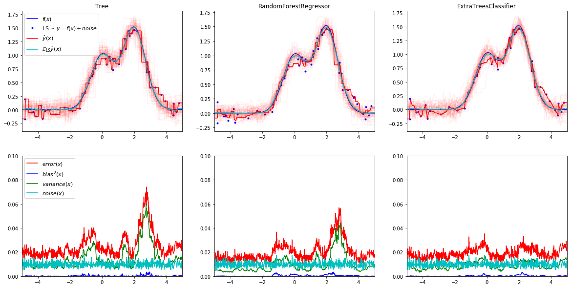
由實驗結果我們可以很好地看出,相對於一般的決策樹,隨機森林雖然增加了模型的偏差,但是大幅度降低了偏差,因而在整體上獲取了更好的結果;而相比之下,在剛剛實驗中的RF演算法方差仍然遠遠大於偏差,這個時候我們就可以採用極限隨機森林,正因為一般而言極限隨機森林相對於隨機森林進一步增加了偏差,同時進一步下降了方差,因為在該實驗中極限隨機森林應當獲取要優於隨機森林的效果(不過這種趨勢並不一定是百分之百的,比如在本次試驗中,極限隨機森林不僅獲取比隨機森林更好的偏差,同時也獲取了更好的方差)
特徵重要程度評估
特徵對於目標變數的相對重要程度,可以根據特徵使用的相對順序進行評估。決策樹頂部使用的特徵對更大一部分輸入樣本的最終預測結果做出貢獻;因此,可以使用接受每個特徵對最終預測的貢獻的樣本比例來評估該 特徵的相對重要性 。
在RF中,通過歲多個隨機數中的預測貢獻率進行平均,降低了方差,因此可用於特徵選擇。不過要注意的是隨機森林與極限隨機森林對於同一個資料集根除的重要程度不一定相同,而且即使是一個模型在引數不同的情況下,最終結果也並不一定相同
因為極限隨機森林的特殊性質,所以請不要採用極限隨機森林進行特徵重要程度的排名,建議使用RF.
import numpy as np
from sklearn.datasets import make_classification
from sklearn.ensemble import ExtraTreesClassifier, RandomForestClassifier
import matplotlib.pyplot as plt

plt.figure(figsize=(8, 4))

estimators = [("RandomForest", RandomForestClassifier(random_state=100)),
              ("ExtraTrees", ExtraTreesClassifier(random_state=100)), ]

n_estimators = len(estimators)

# Build a classification task using 3 informative features
X, y = make_classification(n_samples=1000,
                           n_features=10,
                           n_informative=3,
                           n_redundant=0,
                           n_repeated=0,
                           n_classes=2,
                           random_state=0,
                           shuffle=False)

# Build a forest and compute the feature importances
forest = ExtraTreesClassifier(n_estimators=250,
                              random_state=0)

forest.fit(X, y)

for n, (name, estimator) in enumerate(estimators):
    estimator.fit(X, y)
    importances = estimator.feature_importances_
    std = np.std([tree.feature_importances_ for tree in forest.estimators_],
                 axis=0)
    indices = np.argsort(importances)[::-1]

    # Print the feature ranking
#     print(name +" Feature ranking:")
#     for f in range(X.shape[1]):
#         print("%d. feature %d (%f)" % (f + 1, indices[f], importances[indices[f]]))

    # Plot the feature importances of the forest
    plt.subplot(1, n_estimators, n + 1)
    plt.title(name + " Feature importances")
    plt.bar(range(X.shape[1]), importances[indices],
            color="r", yerr=std[indices], align="center")
    plt.xticks(range(X.shape[1]), indices)
    plt.xlim([-1, X.shape[1]])
plt.show()- 1
- 2
- 3
- 4
- 5
- 6
- 7
- 8
- 9
- 10
- 11
- 12
- 13
- 14
- 15
- 16
- 17
- 18
- 19
- 20
- 21
- 22
- 23
- 24
- 25
- 26
- 27
- 28
- 29
- 30
- 31
- 32
- 33
- 34
- 35
- 36
- 37
- 38
- 39
- 40
- 41
- 42
- 43
- 44
- 45
- 46
- 47
- 48

完全隨機樹嵌入
sklearn中還實現了隨機森林的一種特殊用法,即完全隨機樹嵌入(RandomTreesEmbedding)。RandomTreesEmbedding 實現了一個無監督的資料轉換。 通過由完全隨機樹構成的森林,RandomTreesEmbedding 使用資料最終歸屬的葉子節點的索引值(編號)對資料進行編碼。 該索引以 one-of-K 方式編碼,最終形成一個高維的稀疏二進位制編碼。 這種編碼可以被非常高效地計算出來,並且可以作為其他學習任務的基礎。 編碼的大小和稀疏度可以通過選擇樹的數量和每棵樹的最大深度來確定。對於整合中的每棵樹的每個節點包含一個例項(校對者注:這裡真的沒搞懂)。 編碼的大小(維度)最多為 n_estimators * 2 ** max_depth,即森林中的葉子節點的最大數。
其作用一共有兩種:
1. 非線性降維
2. 生成新的特徵(此處與GBT系列的效果相似,但是生成的新特徵的作用從後面的實驗來看,似乎不如GBT系列)
對於功能一
下面是一個驗證完全隨機樹嵌入作用的兩個例子:
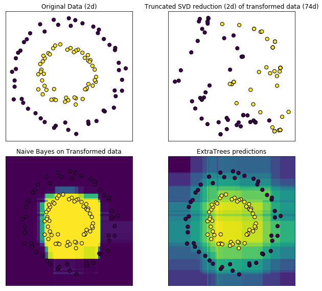
RandomTreesEmbedding提供了一種將資料對映到非常高維稀疏表示的方法,這可能有助於分類。該對映是完全無監督的,非常有效。
這個例子顯示了由幾棵樹給出的分割槽,並且顯示了變換如何也可以用於非線性降維或者非線性分類。
相鄰的點經常共享同一個樹的葉節點並且因此共享大部分的散列表示,這允許截斷奇異值分解(truncated SVD)可以分離資料轉換後的兩個同心圓。
在高維空間中,線性分類器通常達到極好的精度。對於稀疏的二進位制資料,BernoulliNB特別適合。最下面一行將BernoulliNB在變換空間中獲得的決策邊界與在原始資料上學習的ExtraTreesClassifier森林進行比較。
from sklearn.datasets import make_circles
from sklearn.ensemble import RandomTreesEmbedding, ExtraTreesClassifier
from sklearn.decomposition import TruncatedSVD
from sklearn.naive_bayes import BernoulliNB

# make a synthetic dataset
X, y = make_circles(factor=0.5, random_state=0, noise=0.05)

# use RandomTreesEmbedding to transform data
hasher = RandomTreesEmbedding(n_estimators=10, random_state=0, max_depth=3)
X_transformed = hasher.fit_transform(X)

# Visualize result after dimensionality reduction using truncated SVD
svd = TruncatedSVD(n_components=2)
X_reduced = svd.fit_transform(X_transformed)

# Learn a Naive Bayes classifier on the transformed data
nb = BernoulliNB()
nb.fit(X_transformed, y)


# Learn an ExtraTreesClassifier for comparison
trees = ExtraTreesClassifier(max_depth=3, n_estimators=10, random_state=0)
trees.fit(X, y)


# scatter plot of original and reduced data
fig = plt.figure(figsize=(9, 8))

ax = plt.subplot(221)
ax.scatter(X[:, 0], X[:, 1], c=y, s=50, edgecolor='k')
ax.set_title("Original Data (2d)")
ax.set_xticks(())
ax.set_yticks(())

ax = plt.subplot(222)
ax.scatter(X_reduced[:, 0], X_reduced[:, 1], c=y, s=50, edgecolor='k')
ax.set_title("Truncated SVD reduction (2d) of transformed data (%dd)" %
             X_transformed.shape[1])
ax.set_xticks(())
ax.set_yticks(())

# Plot the decision in original space. For that, we will assign a color
# to each point in the mesh [x_min, x_max]x[y_min, y_max].
h = .01
x_min, x_max = X[:, 0].min() - .5, X[:, 0].max() + .5
y_min, y_max = X[:, 1].min() - .5, X[:, 1].max() + .5
xx, yy = np.meshgrid(np.arange(x_min, x_max, h), np.arange(y_min, y_max, h))

# transform grid using RandomTreesEmbedding
transformed_grid = hasher.transform(np.c_[xx.ravel(), yy.ravel()])
y_grid_pred = nb.predict_proba(transformed_grid)[:, 1]

ax = plt.subplot(223)
ax.set_title("Naive Bayes on Transformed data")
ax.pcolormesh(xx, yy, y_grid_pred.reshape(xx.shape))
ax.scatter(X[:, 0], X[:, 1], c=y, s=50, edgecolor='k')
ax.set_ylim(-1.4, 1.4)
ax.set_xlim(-1.4, 1.4)
ax.set_xticks(())
ax.set_yticks(())

# transform grid using ExtraTreesClassifier
y_grid_pred = trees.predict_proba(np.c_[xx.ravel(), yy.ravel()])[:, 1]

ax = plt.subplot(224)
ax.set_title("ExtraTrees predictions")
ax.pcolormesh(xx, yy, y_grid_pred.reshape(xx.shape))
ax.scatter(X[:, 0], X[:, 1], c=y, s=50, edgecolor='k')
ax.set_ylim(-1.4, 1.4)
ax.set_xlim(-1.4, 1.4)
ax.set_xticks(())
ax.set_yticks(())

plt.tight_layout()
plt.show()- 1
- 2
- 3
- 4
- 5
- 6
- 7
- 8
- 9
- 10
- 11
- 12
- 13
- 14
- 15
- 16
- 17
- 18
- 19
- 20
- 21
- 22
- 23
- 24
- 25
- 26
- 27
- 28
- 29
- 30
- 31
- 32
- 33
- 34
- 35
- 36
- 37
- 38
- 39
- 40
- 41
- 42
- 43
- 44
- 45
- 46
- 47
- 48
- 49
- 50
- 51
- 52
- 53
- 54
- 55
- 56
- 57
- 58
- 59
- 60
- 61
- 62
- 63
- 64
- 65
- 66
- 67
- 68
- 69
- 70
- 71
- 72
- 73
- 74
- 75
- 76
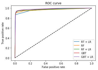
[關於生成新特徵這一作用的實驗](Feature transformations with ensembles of trees)
完全隨機樹嵌入,可以將特徵轉化為更高維度,更稀疏的空間,方式為首先在資料集上訓練模型(極限隨機森林,隨機森林,GBT系列皆可)然後將新的特徵空間中每個葉節點都會分配一個固定的特徵索引,然後將所有的葉節點進行獨熱編碼,通過將樣本所在的葉子設定為1,其他特徵設定為0,來對樣本進行編碼,將其轉轉換到稀疏的,高維度的空間.
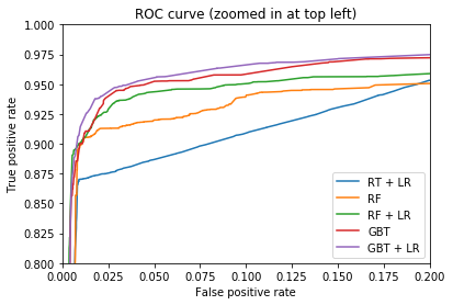
下面的程式碼展示了,不同轉換模型轉換出的特徵最終得到特徵在LR上的分類效果,第二幅圖是第一幅圖左上角的放大,可以看出在本資料集上似乎還是GBT系列的轉換效果好一些(你也可以使用lightGBM與XGBoot中的sklearn藉口,實現程式碼中GradientBoostingClassifier類似的效果)
import numpy as np
np.random.seed(10)

import matplotlib.pyplot as plt

from sklearn.datasets import make_classification
from sklearn.linear_model import LogisticRegression
from sklearn.ensemble import (RandomTreesEmbedding, RandomForestClassifier,
                              GradientBoostingClassifier)
from sklearn.preprocessing import OneHotEncoder
from sklearn.model_selection import train_test_split
from sklearn.metrics import roc_curve
from sklearn.pipeline import make_pipeline

n_estimator = 10
X, y = make_classification(n_samples=80000)
X_train, X_test, y_train, y_test = train_test_split(X, y, test_size=0.5)
# It is important to train the ensemble of trees on a different subset
# of the training data than the linear regression model to avoid
# overfitting, in particular if the total number of leaves is
# similar to the number of training samples
X_train, X_train_lr, y_train, y_train_lr = train_test_split(X_train,
                                                            y_train,
                                                            test_size=0.5)

# Unsupervised transformation based on totally random trees
rt = RandomTreesEmbedding(max_depth=3, n_estimators=n_estimator,
    random_state=0)

rt_lm = LogisticRegression()
pipeline = make_pipeline(rt, rt_lm)
pipeline.fit(X_train, y_train)
y_pred_rt = pipeline.predict_proba(X_test)[:, 1]
fpr_rt_lm, tpr_rt_lm, _ = roc_curve(y_test, y_pred_rt)

# Supervised transformation based on random forests
rf = RandomForestClassifier(max_depth=3, n_estimators=n_estimator)
rf_enc = OneHotEncoder()
rf_lm = LogisticRegression()
rf.fit(X_train, y_train)
rf_enc.fit(rf.apply(X_train))
rf_lm.fit(rf_enc.transform(rf.apply(X_train_lr)), y_train_lr)

y_pred_rf_lm = rf_lm.predict_proba(rf_enc.transform(rf.apply(X_test)))[:, 1]
fpr_rf_lm, tpr_rf_lm, _ = roc_curve(y_test, y_pred_rf_lm)

grd = GradientBoostingClassifier(n_estimators=n_estimator)
grd_enc = OneHotEncoder()
grd_lm = LogisticRegression()
grd.fit(X_train, y_train)
grd_enc.fit(grd.apply(X_train)[:, :, 0])
grd_lm.fit(grd_enc.transform(grd.apply(X_train_lr)[:, :, 0]), y_train_lr)

y_pred_grd_lm = grd_lm.predict_proba(
    grd_enc.transform(grd.apply(X_test)[:, :, 0]))[:, 1]
fpr_grd_lm, tpr_grd_lm, _ = roc_curve(y_test, y_pred_grd_lm)


# The gradient boosted model by itself
y_pred_grd = grd.predict_proba(X_test)[:, 1]
fpr_grd, tpr_grd, _ = roc_curve(y_test, y_pred_grd)


# The random forest model by itself
y_pred_rf = rf.predict_proba(X_test)[:, 1]
fpr_rf, tpr_rf, _ = roc_curve(y_test, y_pred_rf)

plt.figure(1)
plt.plot([0, 1], [0, 1], 'k--')
plt.plot(fpr_rt_lm, tpr_rt_lm, label='RT + LR')
plt.plot(fpr_rf, tpr_rf, label='RF')
plt.plot(fpr_rf_lm, tpr_rf_lm, label='RF + LR')
plt.plot(fpr_grd, tpr_grd, label='GBT')
plt.plot(fpr_grd_lm, tpr_grd_lm, label='GBT + LR')
plt.xlabel('False positive rate')
plt.ylabel('True positive rate')
plt.title('ROC curve')
plt.legend(loc='best')
plt.show()

plt.figure(2)
plt.xlim(0, 0.2)
plt.ylim(0.8, 1)
plt.plot([0, 1], [0, 1], 'k--')
plt.plot(fpr_rt_lm, tpr_rt_lm, label='RT + LR')
plt.plot(fpr_rf, tpr_rf, label='RF')
plt.plot(fpr_rf_lm, tpr_rf_lm, label='RF + LR')
plt.plot(fpr_grd, tpr_grd, label='GBT')
plt.plot(fpr_grd_lm, tpr_grd_lm, label='GBT + LR')
plt.xlabel('False positive rate')
plt.ylabel('True positive rate')
plt.title('ROC curve (zoomed in at top left)')
plt.legend(loc='best')
plt.show()- 1
- 2
- 3
- 4
- 5
- 6
- 7
- 8
- 9
- 10
- 11
- 12
- 13
- 14
- 15
- 16
- 17
- 18
- 19
- 20
- 21
- 22
- 23
- 24
- 25
- 26
- 27
- 28
- 29
- 30
- 31
- 32
- 33
- 34
- 35
- 36
- 37
- 38
- 39
- 40
- 41
- 42
- 43
- 44
- 45
- 46
- 47
- 48
- 49
- 50
- 51
- 52
- 53
- 54
- 55
- 56
- 57
- 58
- 59
- 60
- 61
- 62
- 63
- 64
- 65
- 66
- 67
- 68
- 69
- 70
- 71
- 72
- 73
- 74
- 75
- 76
- 77
- 78
- 79
- 80
- 81
- 82
- 83
- 84
- 85
- 86
- 87
- 88
- 89
- 90
- 91
- 92
- 93
- 94
除此之外,隨機森林還可以進行異常檢測,sklearn中也實現了該演算法IsolationForest.更多內容請閱讀我的部落格。