
使用關鍵點進行小目標檢測
阿新 • • 發佈:2020-09-03
【GiantPandaCV導語】本文是筆者出於興趣搞了一個小的庫,主要是用於定位紅外小目標。由於其具有尺度很小的特點,所以可以嘗試用點的方式代表其位置。本文主要採用了迴歸和heatmap兩種方式來回歸關鍵點,是一個很簡單基礎的專案,程式碼量很小,可供新手學習。
## 1. 資料來源
**資料集**:資料來源自小武,經過小武的授權使用,但不會公開。本專案只用了其中很少一部分共108張圖片。
**標註工具**:https://github.com/pprp/landmark_annotation
> 標註工具也可以在GiantPandaCV公眾號後臺回覆“landmark”關鍵字獲取
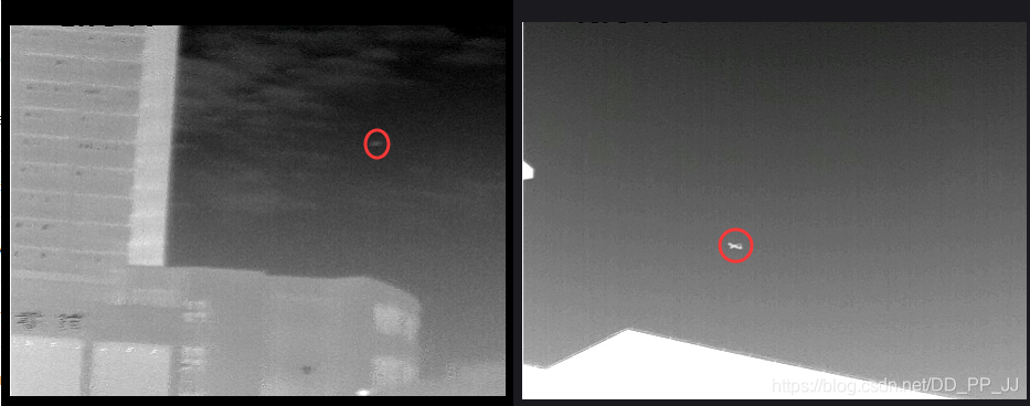
上圖是資料集中的兩張圖片,紅圈代表對應的目標,標註的時候只需要在其中心點一下即可得到該點對應的橫縱座標。
該資料集有一個特點,每張圖只有一個目標(不然沒法用簡單的方法迴歸),多餘一個目標的圖片被剔除了。
```python
1
0.42 0.596
```
以上是一個標註檔案的例子,1.jpg對應1.txt
## 2. 迴歸確定關鍵點
迴歸確定關鍵點比較簡單,網路部分採用手工構建的一個兩層的小網路,訓練採用的是MSELoss。
這部分程式碼在:https://github.com/pprp/SimpleCVReproduction/tree/master/simple_keypoint/regression
### 2.1 資料載入
資料的組織比較簡單,按照以下格式組織:
```tcl
- data
- images
- 1.jpg
- 2.jpg
- ...
- labels
- 1.txt
- 2.txt
- ...
```
重寫一下Dataset類,用於載入資料集。
```python
class KeyPointDatasets(Dataset):
def __init__(self, root_dir="./data", transforms=None):
super(KeyPointDatasets, self).__init__()
self.img_path = os.path.join(root_dir, "images")
# self.txt_path = os.path.join(root_dir, "labels")
self.img_list = glob.glob(os.path.join(self.img_path, "*.jpg"))
self.txt_list = [item.replace(".jpg", ".txt").replace(
"images", "labels") for item in self.img_list]
if transforms is not None:
self.transforms = transforms
def __getitem__(self, index):
img = self.img_list[index]
txt = self.txt_list[index]
img = cv2.imread(img)
if self.transforms:
img = self.transforms(img)
label = []
with open(txt, "r") as f:
for i, line in enumerate(f):
if i == 0:
# 第一行
num_point = int(line.strip())
else:
x1, y1 = [(t.strip()) for t in line.split()]
# range from 0 to 1
x1, y1 = float(x1), float(y1)
tmp_label = (x1, y1)
label.append(tmp_label)
return img, torch.tensor(label[0])
def __len__(self):
return len(self.img_list)
@staticmethod
def collect_fn(batch):
imgs, labels = zip(*batch)
return torch.stack(imgs, 0), torch.stack(labels, 0)
```
返回的結果是圖片和對應座標位置。
### 2.2 網路模型
```python
import torch
import torch.nn as nn
class KeyPointModel(nn.Module):
def __init__(self):
super(KeyPointModel, self).__init__()
self.conv1 = nn.Conv2d(3, 6, 3, 1, 1)
self.bn1 = nn.BatchNorm2d(6)
self.relu1 = nn.ReLU(True)
self.maxpool1 = nn.MaxPool2d((2, 2))
self.conv2 = nn.Conv2d(6, 12, 3, 1, 1)
self.bn2 = nn.BatchNorm2d(12)
self.relu2 = nn.ReLU(True)
self.maxpool2 = nn.MaxPool2d((2, 2))
self.gap = nn.AdaptiveMaxPool2d(1)
self.classifier = nn.Sequential(
nn.Linear(12, 2),
nn.Sigmoid()
)
def forward(self, x):
x = self.conv1(x)
x = self.bn1(x)
x = self.relu1(x)
x = self.maxpool1(x)
x = self.conv2(x)
x = self.bn2(x)
x = self.relu2(x)
x = self.maxpool2(x)
x = self.gap(x)
x = x.view(x.shape[0], -1)
return self.classifier(x)
```
其結構就是卷積+pooling+卷積+pooling+global average pooling+Linear,返回長度為2的tensor。
### 2.3 訓練
```python
def train(model, epoch, dataloader, optimizer, criterion):
model.train()
for itr, (image, label) in enumerate(dataloader):
bs = image.shape[0]
output = model(image)
loss = criterion(output, label)
optimizer.zero_grad()
loss.backward()
optimizer.step()
if itr % 4 == 0:
print("epoch:%2d|step:%04d|loss:%.6f" % (epoch, itr, loss.item()/bs))
vis.plot_many_stack({"train_loss": loss.item()*100/bs})
total_epoch = 300
bs = 10
########################################
transforms_all = transforms.Compose([
transforms.ToPILImage(),
transforms.Resize((360,480)),
transforms.ToTensor(),
transforms.Normalize(mean=[0.4372, 0.4372, 0.4373],
std=[0.2479, 0.2475, 0.2485])
])
datasets = KeyPointDatasets(root_dir="./data", transforms=transforms_all)
data_loader = DataLoader(datasets, shuffle=True,
batch_size=bs, collate_fn=datasets.collect_fn)
model = KeyPointModel()
optimizer = torch.optim.Adam(model.parameters(), lr=3e-4)
# criterion = torch.nn.SmoothL1Loss()
criterion = torch.nn.MSELoss()
scheduler = torch.optim.lr_scheduler.StepLR(optimizer,
step_size=30,
gamma=0.1)
for epoch in range(total_epoch):
train(model, epoch, data_loader, optimizer, criterion)
loss = test(model, epoch, data_loader, criterion)
if epoch % 10 == 0:
torch.save(model.state_dict(),
"weights/epoch_%d_%.3f.pt" % (epoch, loss*1000))
```
loss部分使用Smooth L1 loss或者MSE loss均可。
MSE Loss:
$$
loss(x,y)=\frac{1}{n}\sum(x_i-y_i)^2
$$
Smooth L1 Loss:
$$
smooth_{L_1}(x)=
\begin{cases}
0.5x^2 & if |x|<1 \\
|x|-0.5 & otherwise
\end{cases}
$$
### 2.4 測試結果

## 3. heatmap確定關鍵點
這部分程式碼很多參考了CenterNet,不過曾經嘗試CenterNet中的loss在這個問題上收斂效果不好,所以參考了kaggle人臉關鍵點定位的解決方法,發現使用簡單的MSELoss效果就很好。
### 3.1 資料載入
這部分和CenterNet構建heatmap的過程類似,不過半徑的確定是人工的。因為資料集中的目標都比較小,半徑的範圍最大不超過半徑為30個畫素的圓。
```python
class KeyPointDatasets(Dataset):
def __init__(self, root_dir="./data", transforms=None):
super(KeyPointDatasets, self).__init__()
self.down_ratio = 1
self.img_w = 480 // self.down_ratio
self.img_h = 360 // self.down_ratio
self.img_path = os.path.join(root_dir, "images")
self.img_list = glob.glob(os.path.join(self.img_path, "*.jpg"))
self.txt_list = [item.replace(".jpg", ".txt").replace(
"images", "labels") for item in self.img_list]
if transforms is not None:
self.transforms = transforms
def __getitem__(self, index):
img = self.img_list[index]
txt = self.txt_list[index]
img = cv2.imread(img)
if self.transforms:
img = self.transforms(img)
label = []
with open(txt, "r") as f:
for i, line in enumerate(f):
if i == 0:
# 第一行
num_point = int(line.strip())
else:
x1, y1 = [(t.strip()) for t in line.split()]
# range from 0 to 1
x1, y1 = float(x1), float(y1)
cx, cy = x1 * self.img_w, y1 * self.img_h
heatmap = np.zeros((self.img_h, self.img_w))
draw_umich_gaussian(heatmap, (cx, cy), 30)
return img, torch.tensor(heatmap).unsqueeze(0)
def __len__(self):
return len(self.img_list)
@staticmethod
def collect_fn(batch):
imgs, labels = zip(*batch)
return torch.stack(imgs, 0), torch.stack(labels, 0)
```
核心函式是draw_umich_gaussian,具體如下:
```python
def gaussian2D(shape, sigma=1):
m, n = [(ss - 1.) / 2. for ss in shape]
y, x = np.ogrid[-m:m + 1, -n:n + 1]
h = np.exp(-(x * x + y * y) / (2 * sigma * sigma))
h[h < np.finfo(h.dtype).eps * h.max()] = 0
# 限制最小的值
return h
def draw_umich_gaussian(heatmap, center, radius, k=1):
diameter = 2 * radius + 1
gaussian = gaussian2D((diameter, diameter), sigma=diameter / 6)
# 一個圓對應內切正方形的高斯分佈
x, y = int(center[0]), int(center[1])
width, height = heatmap.shape
left, right = min(x, radius), min(width - x, radius + 1)
top, bottom = min(y, radius), min(height - y, radius + 1)
masked_heatmap = heatmap[y - top:y + bottom, x - left:x + right]
masked_gaussian = gaussian[radius - top:radius +
bottom, radius - left:radius + right]
if min(masked_gaussian.shape) >