深度學習BP演算法 BackPropagation以及詳細例子解析

阿新 • • 發佈：2018-11-05

反向傳播演算法是多層神經網路的訓練中舉足輕重的演算法，本文著重講解方向傳播演算法的原理和推導過程。因此對於一些基本的神經網路的知識，本文不做介紹。在理解反向傳播演算法前，先要理解神經網路中的前饋神經網路演算法。

前饋神經網路

如下圖，是一個多層神經網路的簡單示意圖：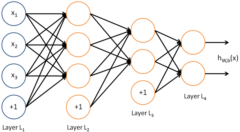
這裡寫圖片描述
給定一個前饋神經網路，我們用下面的記號來描述這個網路：
L：表示神經網路的層數；
nl：表示第l層神經元的個數；
fl(∙)：表示l層神經元的啟用函式；
Wl∈Rnl×nl−1：表示l−1層到第l層的權重矩陣；
bl∈Rnl：表示l−

1層到

l層的偏置；

zl∈Rnl：表示第

l層神經元的輸入；

al∈Rnl：表示第

l層神經元的輸出；

前饋神經網路通過如下的公式進行資訊傳播：

zl=Wl⋅al−1+blal=fl(zl) 上述兩個公式可以合併寫成如下形式：

zl=Wl⋅fl(zl−1)+bl 這樣通過一層一層的資訊傳遞，可以得到網路的最後輸出

y為：

x=a0→z1→a1→z1→⋯→aL−1→zL→aL=y

反向傳播演算法

在瞭解前饋神經網路的結構之後，我們一前饋神經網路的資訊傳遞過程為基礎，從而推到反向傳播演算法。首先要明確一點，反向傳播演算法是為了更好更快的訓練前饋神經網路，得到神經網路每一層的權重引數和偏置引數。
在推導反向傳播的理論之前，首先看一幅能夠直觀的反映反向傳播過程的圖，這個圖取材於Principles of training multi-layer neural network using back propagation。

Principles of training multi-layer neural network using backpropagation

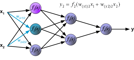
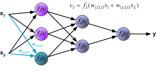
The project describes teaching process of multi-layer neural network employing backpropagation algorithm. To illustrate this process the three layer neural network with two inputs and one output,which is shown in the picture below, is used: 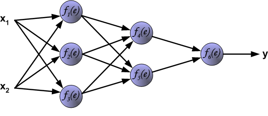Each neuron is composed of two units. First unit adds products of weights coefficients and input signals. The second unit realise nonlinear function, called neuron activation function. Signal e is adder output signal, and y = f(e) is output signal of nonlinear element. Signal y is also output signal of neuron. 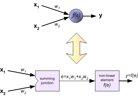To teach the neural network we need training data set. The training data set consists of input signals (x₁ and x₂ ) assigned with corresponding target (desired output) z. The network training is an iterative process. In each iteration weights coefficients of nodes are modified using new data from training data set. Modification is calculated using algorithm described below: Each teaching step starts with forcing both input signals from training set. After this stage we can determine output signals values for each neuron in each network layer. Pictures below illustrate how signal is propagating through the network, Symbols w_(xm)n represent weights of connections between network input x_m and neuron n in input layer. Symbols y_n represents output signal of neuron n. 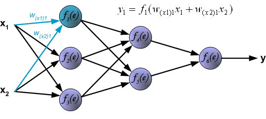Propagation of signals through the hidden layer. Symbols w_mn represent weights of connections between output of neuron m and input of neuron n in the next layer. 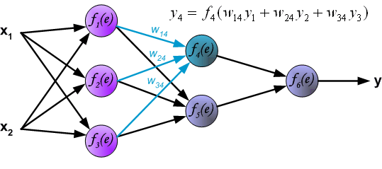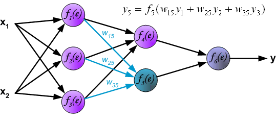Propagation of signals through the output layer. 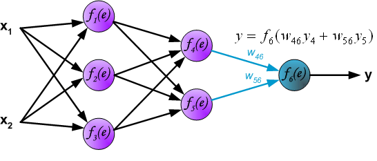In the next algorithm step the output signal of the network y is compared with the desired output value (the target), which is found in training data set. The difference is called error signal d of output layer neuron. 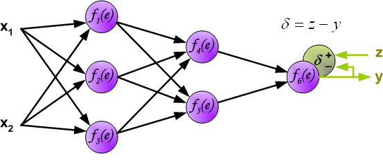It is impossible to compute error signal for internal neurons directly, because output values of these neurons are unknown. For many years the effective method for training multiplayer networks has been unknown. Only in the middle eighties the backpropagation algorithm has been worked out. The idea is to propagate error signal d (computed in single teaching step) back to all neurons, which output signals were input for discussed neuron. 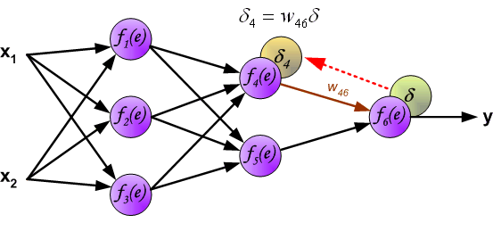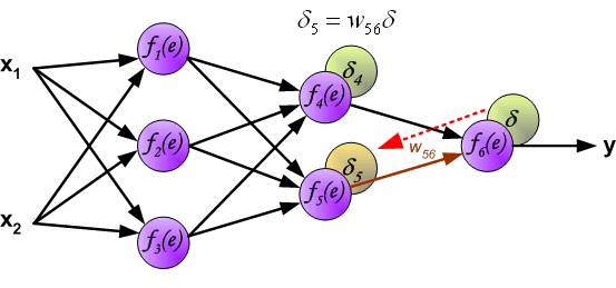The weights' coefficients w_mn used to propagate errors back are equal to this used during computing output value. Only the direction of data flow is changed (signals are propagated from output to inputs one after the other). This technique is used for all network layers. If propagated errors came from few neurons they are added. 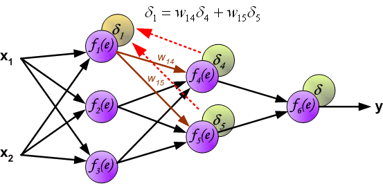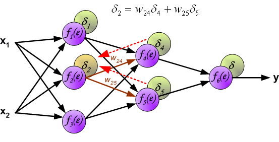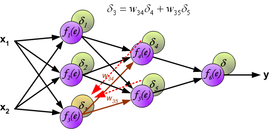The illustration is below: When the error signal for each neuron is computed, the weights coefficients of each neuron input node may be modified. In formulas below df(e)/de represents derivative of neuron activation function (which weights are modified). 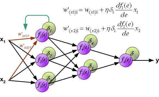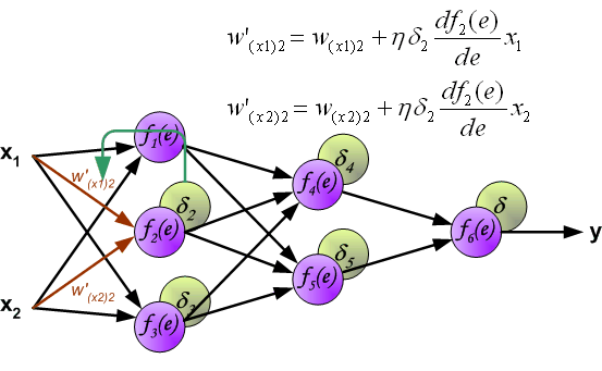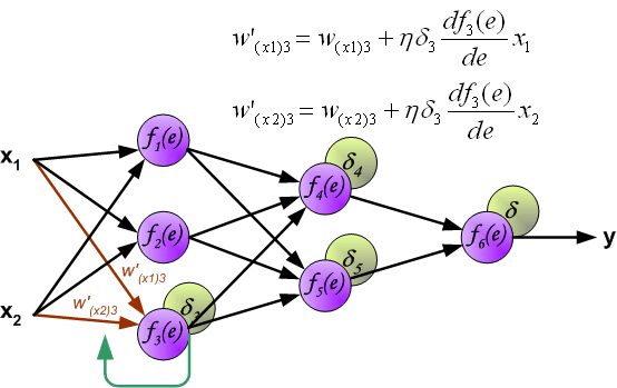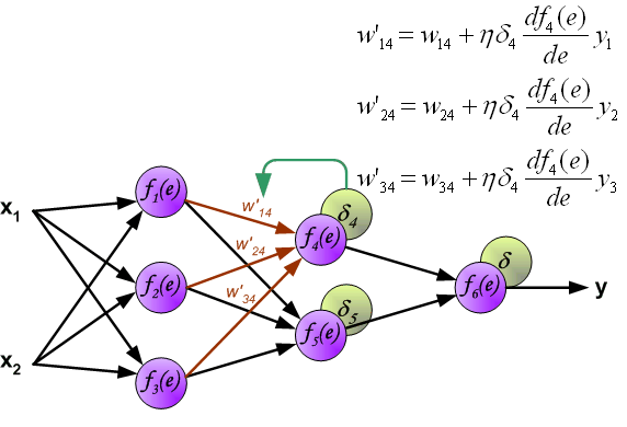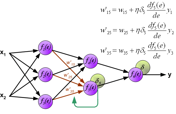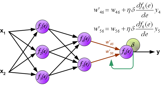Coefficient h affects network teaching speed. There are a few techniques to select this parameter. The first method is to start teaching process with large value of the parameter. While weights coefficients are being established the parameter is being decreased gradually. The second, more complicated, method starts teaching with small parameter value. During the teaching process the parameter is being increased when the teaching is advanced and then decreased again in the final stage. Starting teaching process with low parameter value enables to determine weights coefficients signs. References Ryszard Tadeusiewcz "Sieci neuronowe", Kraków 1992

Mariusz Bernacki Przemysław Włodarczyk mgr inż. Adam Gołda (2005) Katedra Elektroniki AGH
Last modified: 06.09.2004 Webmaster

A Step by Step Backpropagation Example

Background

Backpropagation is a common method for training a neural network. There is no shortage of papers online that attempt to explain how backpropagation works, but few that include an example with actual numbers. This post is my attempt to explain how it works with a concrete example that folks can compare their own calculations to in order to ensure they understand backpropagation correctly.

If this kind of thing interests you, you should sign up for my newsletter where I post about AI-related projects that I’m working on.

Backpropagation in Python

You can play around with a Python script that I wrote that implements the backpropagation algorithm in this Github repo.

Backpropagation Visualization

For an interactive visualization showing a neural network as it learns, check out my Neural Network visualization.

Additional Resources

If you find this tutorial useful and want to continue learning about neural networks and their applications, I highly recommend checking out Adrian Rosebrock’s excellent tutorial on Getting Started with Deep Learning and Python.

Overview

For this tutorial, we’re going to use a neural network with two inputs, two hidden neurons, two output neurons. Additionally, the hidden and output neurons will include a bias.

Here’s the basic structure:

neural_network (7)

In order to have some numbers to work with, here are the initial weights, the biases, and training inputs/outputs:

neural_network (9)

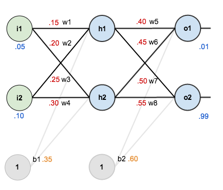
The goal of backpropagation is to optimize the weights so that the neural network can learn how to correctly map arbitrary inputs to outputs.

For the rest of this tutorial we’re going to work with a single training set: given inputs 0.05 and 0.10, we want the neural network to output 0.01 and 0.99.

The Forward Pass

To begin, lets see what the neural network currently predicts given the weights and biases above and inputs of 0.05 and 0.10. To do this we’ll feed those inputs forward though the network.

We figure out the total net input to each hidden layer neuron, squash the total net input using an activation function (here we use the logistic function), then repeat the process with the output layer neurons.

Total net input is also referred to as just net input by some sources.

Here’s how we calculate the total net input for $h_1$ :

$net_{h1} = w_1 * i_1 + w_2 * i_2 + b_1 * 1$

$net_{h1} = 0.15 * 0.05 + 0.2 * 0.1 + 0.35 * 1 = 0.3775$

We then squash it using the logistic function to get the output of $h_1$ :

$out_{h1} = \frac{1}{1+e^{-net_{h1}}} = \frac{1}{1+e^{-0.3775}} = 0.593269992$

Carrying out the same process for $h_2$ we get:

$out_{h2} = 0.596884378$

We repeat this process for the output layer neurons, using the output from the hidden layer neurons as inputs.

Here’s the output for $o_1$ :

$net_{o1} = w_5 * out_{h1} + w_6 * out_{h2} + b_2 * 1$

$net_{o1} = 0.4 * 0.593269992 + 0.45 * 0.596884378 + 0.6 * 1 = 1.105905967$

$out_{o1} = \frac{1}{1+e^{-net_{o1}}} = \frac{1}{1+e^{-1.105905967}} = 0.75136507$

And carrying out the same process for $o_2$ we get:

$out_{o2} = 0.772928465$

Calculating the Total Error

We can now calculate the error for each output neuron using the squared error function and sum them to get the total error:

$E_{total} = \sum \frac{1}{2}(target - output)^{2}$

Some sources refer to the target as the ideal and the output as the actual. The $\frac{1}{2}$ is included so that exponent is cancelled when we differentiate later on. The result is eventually multiplied by a learning rate anyway so it doesn’t matter that we introduce a constant here [ 1].

For example, the target output for $o_1$ is 0.01 but the neural network output 0.75136507, therefore its error is:

$E_{o1} = \frac{1}{2}(target_{o1} - out_{o1})^{2} = \frac{1}{2}(0.01 - 0.75136507)^{2} = 0.274811083$

Repeating this process for $o_2$ (remembering that the target is 0.99) we get:

$E_{o2} = 0.023560026$

The total error for the neural network is the sum of these errors:

$E_{total} = E_{o1} + E_{o2} = 0.274811083 + 0.023560026 = 0.298371109$

The Backwards Pass

Our goal with backpropagation is to update each of the weights in the network so that they cause the actual output to be closer the target output, thereby minimizing the error for each output neuron and the network as a whole.

Output Layer

Consider $w_5$ . We want to know how much a change in $w_5$ affects the total error, aka $\frac{\partial E_{total}}{\partial w_{5}}$ .

$\frac{\partial E_{total}}{\partial w_{5}}$ is read as “the partial derivative of $E_{total}$ with respect to $w_{5}$ “. You can also say “the gradient with respect to $w_{5}$ “.

By applying the chain rule we know that:

$\frac{\partial E_{total}}{\partial w_{5}} = \frac{\partial E_{total}}{\partial out_{o1}} * \frac{\partial out_{o1}}{\partial net_{o1}} * \frac{\partial net_{o1}}{\partial w_{5}}$

Visually, here’s what we’re doing:

output_1_backprop (4)

We need to figure out each piece in this equation.

First, how much does the total error change with respect to the output?

$E_{total} = \frac{1}{2}(target_{o1} - out_{o1})^{2} + \frac{1}{2}(target_{o2} - out_{o2})^{2}$

$\frac{\partial E_{total}}{\partial out_{o1}} = 2 * \frac{1}{2}(target_{o1} - out_{o1})^{2 - 1} * -1 + 0$

$\frac{\partial E_{total}}{\partial out_{o1}} = -(target_{o1} - out_{o1}) = -(0.01 - 0.75136507) = 0.74136507$

$-(target - out)$ is sometimes expressed as $out - target$ When we take the partial derivative of the total error with respect to $out_{o1}$ , the quantity $\frac{1}{2}(target_{o2} - out_{o2})^{2}$ becomes zero because $out_{o1}$ does not affect it which means we’re taking the derivative of a constant which is zero.

Next, how much does the output of $o_1$ change with respect to its total net input?

The partial derivative of the logistic function is the output multiplied by 1 minus the output:

$out_{o1} = \frac{1}{1+e^{-net_{o1}}}$

$\frac{\partial out_{o1}}{\partial net_{o1}} = out_{o1}(1 - out_{o1}) = 0.75136507(1 - 0.75136507) = 0.186815602$

Finally, how much does the total net input of $o1$ change with respect to $w_5$ ?

$net_{o1} = w_5 * out_{h1} + w_6 * out_{h2} + b_2 * 1$

$\frac{\partial net_{o1}}{\partial w_{5}} = 1 * out_{h1} * w_5^{(1 - 1)} + 0 + 0 = out_{h1} = 0.593269992$

Putting it all together:

$\frac{\partial E_{total}}{\partial w_{5}} = \frac{\partial E_{total}}{\partial out_{o1}} * \frac{\partial out_{o1}}{\partial net_{o1}} * \frac{\partial net_{o1}}{\partial w_{5}}$

$\frac{\partial E_{total}}{\partial w_{5}} = 0.74136507 * 0.186815602 * 0.593269992 = 0.082167041$

You’ll often see this calculation combined in the form of the delta rule:

$\frac{\partial E_{total}}{\partial w_{5}} = -(target_{o1} - out_{o1}) * out_{o1}(1 - out_{o1}) * out_{h1}$

Alternatively, we have $\frac{\partial E_{total}}{\partial out_{o1}}$ and $\frac{\partial out_{o1}}{\partial net_{o1}}$ which can be written as $\frac{\partial E_{total}}{\partial net_{o1}}$ , aka $\delta_{o1}$ (t

深度學習BP演算法 BackPropagation以及詳細例子解析

前饋神經網路

反向傳播演算法

Principles of training multi-layer neural network using backpropagation

A Step by Step Backpropagation Example

Background

Backpropagation in Python

Backpropagation Visualization

Additional Resources

Overview

The Forward Pass

Calculating the Total Error

The Backwards Pass

Output Layer

深度學習BP演算法 BackPropagation以及詳細例子解析

深度學習 --- BP演算法詳解（誤差反向傳播演算法）

深度學習 --- BP演算法詳解（BP演算法的優化）

深度學習 --- BP演算法詳解（流程圖、BP主要功能、BP演算法的侷限性）

286頁PDF教你如何搞明白深度學習的演算法、理論與計算系統！(可下載)

深度學習優化演算法：動量、RMSProp、Adam

機器學習&深度學習優化演算法

強化學習Sarsa演算法走迷宮小例子

[深度學習] 優化演算法

深度學習CNN演算法原理

深度學習常見演算法介紹與比較

深度學習Loss 種類彙總以及討論

吳恩達深度學習——優化演算法

DAY7: 神經網路及深度學習基礎--演算法的優化（deeplearning.ai）

主要推薦系統演算法總結及Youtube深度學習推薦演算法例項概括

GOTURN-(達到100FPS的深度學習跟蹤演算法程式碼)

2017年深度學習優化演算法最新進展：改進SGD和Adam方法

2017年深度學習優化演算法最新綜述

深度學習優化演算法總結

深度學習優化演算法總結與實驗

深度學習BP演算法 BackPropagation以及詳細例子解析

前饋神經網路

反向傳播演算法

Principles of training multi-layer neural network using backpropagation

A Step by Step Backpropagation Example

Background

Backpropagation in Python

Backpropagation Visualization

Additional Resources

Overview

The Forward Pass

Calculating the Total Error

The Backwards Pass

Output Layer

相關推薦