
深度學習第二課 Softmax迴歸
阿新 • • 發佈:2018-11-11
與第一課線性迴歸(linear regression)不同,softmax迴歸針對的是多分類的情況,即labels不再僅有0,1兩個分類。
softmax通過指數運算將最後的分類轉為0~1間的概率,在終於類別概率中,數值大的為預測概率。
與線性迴歸損失不同,softmax函式計算損失採用的是交叉熵損失(Cross Entropy),原理和公式推導可參考:https://zhuanlan.zhihu.com/p/27223959
softmax函式簡單實現程式碼如下:
from mxnet import autograd,nd
import gluonbook as gb
%matplotlib inline
import time
import matplotlib.pyplot as plt
import sys

#讀取資料
batch_size = 256
train_iter,test_iter = gb.load_data_fashion_mnist(batch_size)

#引數初始化
num_inputs = 784
num_outputs = 10

w = nd.random.normal(scale = 1,shape = (num_inputs,num_outputs))
b = nd.random.normal(num_outputs)

w.attach_grad()
b.attach_grad()

#正向傳播,實現softmax運算
def softmax(x):
    return nd.exp(x) / nd.exp(x).sum(axis = 1,keepdims = True)

def net(x):
    return softmax(nd.dot(x.reshape((-1,num_inputs)),w) + b)    #對求得的yhat執行softmax運算

def cross_entropy(y_hat,y):               #定義交叉損失熵函式
    return -nd.pick(y_hat,y).log()
def accuracy(yhat,y):
    return (yhat.argmax(axis = 1) == y.astype('float32')).mean().asscalar()   #提取yhat中每行概率最大的類別和真實值y的類別比較後的概率
def evaluate_accuracy(data_iter,net):
    acc = 0
    for X,y in data_iter:
        acc+= accuracy(net(X),y)
        return acc/len(data_iter)

num_epochs,lr = 5,0.1
#訓練模型
def train_ch3(net,train_iter,test_iter,loss,num_epochs,batch_size,params = None,lr = None,trainer = None):
    for epoch in range(num_epochs):
        train_l_sum = 0     #定義訓練損失總和
        train_acc_sum = 0   #定義訓練精度總和
        for X ,y in train_iter:
            with autograd.record():
                y_hat = net(X)
                l = loss(y_hat,y)
            l.backward()
            if trainer is None:
                gb.sgd(params,lr,batch_size)
            else:
                trainer.step(batch_size)
            train_l_sum += l.mean().asscalar()
            train_acc_sum += accuracy(y_hat,y)
        test_acc = evaluate_accuracy(test_iter,net)
        print('epoch %d, loss %.4f, train acc %.3f, test acc %.3f'
              % (epoch + 1, train_l_sum / len(train_iter),
                 train_acc_sum / len(train_iter), test_acc))
train_ch3(net, train_iter, test_iter, cross_entropy, num_epochs,
          batch_size, [w, b], lr)
簡單小計:
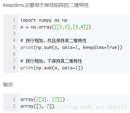
1)keepdims = True:
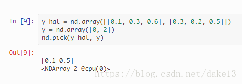
2)nd.pick():
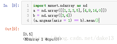
3) (yhat.argmax(axis = 1) == y.astype('float32')).mean().asscalar():
取yhat中每行概率最大的類別和真實值y的類別比較後的概率(比較後得到的矩陣裡面只有0和1兩類),.mean()相當於求取了和真實值比較多概率。
eg:
Softmax()的Gluon實現:
%matplotlib inline
import gluonbook as gb
from mxnet import gluon, init
from mxnet.gluon import loss as gloss, nn

#讀取資料
batch_size = 256
train_iter, test_iter = gb.load_data_fashion_mnist(batch_size)

#初始化模型
net = nn.Sequential()
net.add(nn.Dense(10))    #定義輸出層目標為10
net.initialize(init.Normal(sigma=0.01))

#定義Softmax函式和損失
loss = gloss.SoftmaxCrossEntropyLoss()
#定義優化演算法
trainer = gluon.Trainer(net.collect_params(), 'sgd', {'learning_rate': 0.1})
#訓練模型
num_epochs = 5
gb.train_ch3(net, train_iter, test_iter, loss, num_epochs, batch_size, None,
             None, trainer)
小計:
1)nn模組:
“nn”是 neural networks(神經網路)的縮寫。顧名思義,該模組定義了大量神經網路的層。我們先定義一個模型變數net,它是一個 Sequential 例項。在 Gluon 中,Sequential 例項可以看作是一個串聯各個層的容器。在構造模型時,我們在該容器中依次新增層。當給定輸入資料時,容器中的每一層將依次計算並將輸出作為下一層的輸入。
作為一個單層神經網路,線性迴歸輸出層中的神經元和輸入層中各個輸入完全連線。因此,線性迴歸的輸出層又叫全連線層。在 Gluon 中,全連線層是一個Dense例項。net.add(nn.Dense(10)),表明輸出層個數是10。