• 機器學習之KPCA降維

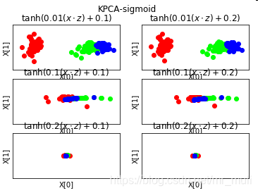
# -*- coding: utf-8 -*-
"""
Created on Sun Nov 25 21:30:48 2018

@author: muli
"""

import numpy as np
import matplotlib.pyplot as plt
from sklearn import  datasets,decomposition


def load_data():
    '''
    載入用於降維的資料

    :return: 一個元組，依次為訓練樣本集和樣本集的標記
    '''
    iris=datasets.load_iris()# 使用 scikit-learn 自帶的 iris 資料集
    return  iris.data,iris.target


def test_KPCA(*data):
    '''
    測試 KernelPCA 的用法

    :param data: 可變引數。
    它是一個元組，這裡要求其元素依次為：訓練樣本集、訓練樣本的標記
    :return: None
    '''
    X,y=data
    kernels=['linear','poly','rbf','sigmoid']
    for kernel in kernels:
        kpca=decomposition.KernelPCA(n_components=None,kernel=kernel) # 依次測試四種核函式
        kpca.fit(X)
        print(np.shape(kpca.lambdas_))
        print("-----------")
        print('kernel=%s --> lambdas: %s'% (kernel,kpca.lambdas_))


def plot_KPCA(*data):
    '''
    繪製經過 KernelPCA 降維到二維之後的樣本點

    :param data: 可變引數。它是一個元組，這裡要求其元素依次為：訓練樣本集、訓練樣本的標記
    :return: None
    '''
    X,y=data
    kernels=['linear','poly','rbf','sigmoid']
    fig=plt.figure()
    colors=((1,0,0),(0,1,0),(0,0,1),(0.5,0.5,0),(0,0.5,0.5),(0.5,0,0.5),
        (0.4,0.6,0),(0.6,0.4,0),(0,0.6,0.4),(0.5,0.3,0.2),)# 顏色集合，不同標記的樣本染不同的顏色

    for i,kernel in enumerate(kernels):
        kpca=decomposition.KernelPCA(n_components=2,kernel=kernel)
        kpca.fit(X)
        # 原始資料集轉換到二維
        X_r=kpca.transform(X)
        ax=fig.add_subplot(2,2,i+1) ## 兩行兩列，每個單元顯示一種核函式的 KernelPCA 的效果圖
        for label ,color in zip( np.unique(y),colors):
            position=y==label
            ax.scatter(X_r[position,0],X_r[position,1],label="target= %d"%label,
            color=color)
        ax.set_xlabel("X[0]")
        ax.set_ylabel("X[1]")
#        ax.legend(loc="best")
        ax.set_title("kernel=%s"%kernel)
    plt.suptitle("KPCA")
    plt.show()


def plot_KPCA_poly(*data):
    '''
    繪製經過 使用 poly 核的KernelPCA 降維到二維之後的樣本點

    :param data: 可變引數。
    它是一個元組，這裡要求其元素依次為：訓練樣本集、訓練樣本的標記
    :return: None
    '''
    X,y=data
    fig=plt.figure()
    colors=((1,0,0),(0,1,0),(0,0,1),(0.5,0.5,0),(0,0.5,0.5),(0.5,0,0.5),
        (0.4,0.6,0),(0.6,0.4,0),(0,0.6,0.4),(0.5,0.3,0.2),)# 顏色集合，不同標記的樣本染不同的顏色
    Params=[(3,1,1),(3,10,1),(3,1,10),(3,10,10),(10,1,1),(10,10,1),(10,1,10),(3,3,1)] # poly 核的引數組成的列表。
            # 每個元素是個元組，代表一組引數（依次為：p 值， gamma 值， r 值）
            # p 取值為：3，10
            # gamma 取值為 ：1，10
            # r 取值為：1，10
            # 排列組合一共 8 種組合
    for i,(p,gamma,r) in enumerate(Params):
        kpca=decomposition.KernelPCA(n_components=2,kernel='poly'
        ,gamma=gamma,degree=p,coef0=r)  # poly 核，目標為2維
        kpca.fit(X)
        X_r=kpca.transform(X)# 原始資料集轉換到二維
        ax=fig.add_subplot(2,4,i+1)## 兩行四列，每個單元顯示核函式為 poly 的 KernelPCA 一組引數的效果圖
        for label ,color in zip( np.unique(y),colors):
            position=y==label
            ax.scatter(X_r[position,0],X_r[position,1],label="target= %d"%label,
            color=color)
        ax.set_xlabel("X[0]")
        ax.set_xticks([]) # 隱藏 x 軸刻度
        ax.set_yticks([]) # 隱藏 y 軸刻度
        ax.set_ylabel("X[1]")
#        ax.legend(loc="best")
        ax.set_title(r"$ (%s (x \cdot z+1)+%s)^{%s}$"%(gamma,r,p))
    plt.suptitle("KPCA-Poly")
    plt.show()


def plot_KPCA_rbf(*data):
    '''
    繪製經過 使用 rbf 核的KernelPCA 降維到二維之後的樣本點

    :param data: 可變引數。它是一個元組，這裡要求其元素依次為：訓練樣本集、訓練樣本的標記
    :return: None
    '''
    X,y=data
    fig=plt.figure()
    colors=((1,0,0),(0,1,0),(0,0,1),(0.5,0.5,0),(0,0.5,0.5),(0.5,0,0.5),
        (0.4,0.6,0),(0.6,0.4,0),(0,0.6,0.4),(0.5,0.3,0.2),)# 顏色集合，不同標記的樣本染不同的顏色
    Gammas=[0.5,1,4,10]# rbf 核的引數組成的列表。每個引數就是 gamma值
    for i,gamma in enumerate(Gammas):
        kpca=decomposition.KernelPCA(n_components=2,kernel='rbf',gamma=gamma)
        kpca.fit(X)
        X_r=kpca.transform(X)# 原始資料集轉換到二維
        ax=fig.add_subplot(2,2,i+1)## 兩行兩列，每個單元顯示核函式為 rbf 的 KernelPCA 一組引數的效果圖
        for label ,color in zip( np.unique(y),colors):
            position=y==label
            ax.scatter(X_r[position,0],X_r[position,1],label="target= %d"%label,
            color=color)
        ax.set_xlabel("X[0]")
        ax.set_xticks([]) # 隱藏 x 軸刻度
        ax.set_yticks([]) # 隱藏 y 軸刻度
        ax.set_ylabel("X[1]")
#        ax.legend(loc="best")
        ax.set_title(r"$\exp(-%s||x-z||^2)$"%gamma)
    plt.suptitle("KPCA-rbf")
    plt.show()


def plot_KPCA_sigmoid(*data):
    '''
    繪製經過 使用 sigmoid 核的KernelPCA 降維到二維之後的樣本點

    :param data: 可變引數。它是一個元組，這裡要求其元素依次為：訓練樣本集、訓練樣本的標記
    :return: None
    '''
    X,y=data
    fig=plt.figure()
    colors=((1,0,0),(0,1,0),(0,0,1),(0.5,0.5,0),(0,0.5,0.5),(0.5,0,0.5),
        (0.4,0.6,0),(0.6,0.4,0),(0,0.6,0.4),(0.5,0.3,0.2),)# 顏色集合，不同標記的樣本染不同的顏色
    Params=[(0.01,0.1),(0.01,0.2),(0.1,0.1),(0.1,0.2),(0.2,0.1),(0.2,0.2)]# sigmoid 核的引數組成的列表。
        # 每個元素就是一種引數組合（依次為 gamma,coef0）
        # gamma 取值為： 0.01，0.1，0.2
        # coef0 取值為： 0.1,0.2
        # 排列組合一共有 6 種組合
    for i,(gamma,r) in enumerate(Params):
        kpca=decomposition.KernelPCA(n_components=2,kernel='sigmoid',gamma=gamma,coef0=r)
        kpca.fit(X)
        X_r=kpca.transform(X)# 原始資料集轉換到二維
        ax=fig.add_subplot(3,2,i+1)## 三行兩列，每個單元顯示核函式為 sigmoid 的 KernelPCA 一組引數的效果圖
        for label ,color in zip( np.unique(y),colors):
            position=y==label
            ax.scatter(X_r[position,0],X_r[position,1],label="target= %d"%label,
            color=color)
        ax.set_xlabel("X[0]")
        ax.set_xticks([]) # 隱藏 x 軸刻度
        ax.set_yticks([]) # 隱藏 y 軸刻度
        ax.set_ylabel("X[1]")
#        ax.legend(loc="best")
        ax.set_title(r"$\tanh(%s(x\cdot z)+%s)$"%(gamma,r))
    plt.suptitle("KPCA-sigmoid")
    plt.show()
    

if __name__=='__main__':
    X,y=load_data() # 產生用於降維的資料集
#    test_KPCA(X,y)   # 呼叫 test_KPCA
#    plot_KPCA(X,y)   # 呼叫 plot_KPCA
#    plot_KPCA_poly(X,y)   # 呼叫 plot_KPCA_poly
#    plot_KPCA_rbf(X,y)   # 呼叫 plot_KPCA_rbf
    plot_KPCA_sigmoid(X,y)   # 呼叫 plot_KPCA_sigmoid

 

• 如圖：