
《CS224n斯坦福課程》-----第一部分的大作業
看到簡化版的題目,我覺得我就像一個腦殘,根本看不懂,只有看到原題目,我才知道要做啥。我現在把原題目貼出來,然後一一的解答。

題目意思:
(a) 證明softmax函式的一個性質,在輸入中存在偏移,但softmax的值是不隨著偏移而改變。在實踐中,我們認為這個偏移值一般是輸入中的最大值。
(b) 給出輸入矩陣,N行D列,然後計算每行的softmax函式值,最好是採用向量化來實現,以便為後續提供一個好的基礎。一個非向量化實現的方式,不會得到全部的分數。
解答二個部分:
(a)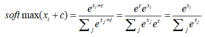
根據指數函式的性質,可以得到此偏移不變形。
(b)程式設計實現
在這個問題中,我們需要主要的幾點:
1,在處理此類問題的時候,向量化操作真的很重要,所以能向量化就向量化,當然對於初學者來說,這種向量化的思路可能剛開始很難理解,但需要不斷的熟悉這種思想,然後不斷的去應用。在向量化中,必不可少的一個庫就是numpy。
numpy的學習網站:https://www.jianshu.com/p/358948fbbc6e
2,在這個問題中,一個技巧,就是利用到了上一步的偏移以及trick,就是這個偏移值是最大的值,否則在官網給出的測試用例就會有溢位的問題。
import numpy as np

def softmax(x):
    """Compute the softmax function for each row of the input x.

    It is crucial that this function is optimized for speed because
    it will be used frequently in later code. You might find numpy
    functions np.exp, np.sum, np.reshape, np.max, and numpy
    broadcasting useful for this task.

    Numpy broadcasting documentation:
    http://docs.scipy.org/doc/numpy/user/basics.broadcasting.html

    You should also make sure that your code works for a single
    D-dimensional vector (treat the vector as a single row) and
    for N x D matrices. This may be useful for testing later. Also,
    make sure that the dimensions of the output match the input.

    You must implement the optimization in problem 1(a) of the
    written assignment!

    Arguments:
    x -- A D dimensional vector or N x D dimensional numpy matrix.

    Return:
    x -- You are allowed to modify x in-place
    """
    orig_shape = x.shape

    if len(x.shape) > 1:
        # Matrix
        x = x - np.max(x, axis=1, keepdims=True)
        x = np.exp(x)/np.sum(np.exp(x), axis=1, keepdims=True)
    else:
        # Vector
        x = x - np.max(x)
        x = np.exp(x)/np.sum(np.exp(x))

    assert x.shape == orig_shape
    return x

def test_softmax_basic():
    """
    Some simple tests to get you started.
    Warning: these are not exhaustive.
    """
    print "Running basic tests..."
    test1 = softmax(np.array([1,2]))
    print test1
    ans1 = np.array([0.26894142,  0.73105858])
    assert np.allclose(test1, ans1, rtol=1e-05, atol=1e-06)

    test2 = softmax(np.array([[1001,1002],[3,4]]))
    print test2
    ans2 = np.array([
        [0.26894142, 0.73105858],
        [0.26894142, 0.73105858]])
    assert np.allclose(test2, ans2, rtol=1e-05, atol=1e-06)

    test3 = softmax(np.array([[-1001,-1002]]))
    print test3
    ans3 = np.array([0.73105858, 0.26894142])
    assert np.allclose(test3, ans3, rtol=1e-05, atol=1e-06)

    print "You should be able to verify these results by hand!\n"


if __name__ == "__main__":
    test_softmax_basic()
測試結果:
我把最後一個print註釋掉了,截圖如下:

手工去測試一下程式:對於指數函式而言,影象如下:

所以對於數值很大的情況,數值可以說很爆炸了,對於數值很小的情況,又太小了,所以採用偏移不變性是一個很好的解決措施。
對於程式裡,老師給出的框架中,assert是做斷言,用於捕捉錯誤資訊,看是否計算出來的數值與真實的數值相差的情況。

題目解釋:
(a)推導sigmod函式的梯度,並且將其寫成複合函式的形式。假定輸入的x是標量。
(b)推導梯度下降(採用交叉熵的softmax函式), 此時class label可以視為0-1的one-hot編碼形式,也就是隻有一個1,其餘均為0。
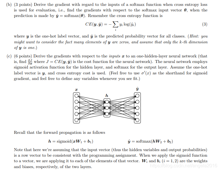
(c)推導梯度下降,輸入x,只有一層隱藏層的神經網路,損失函式利用交叉熵來度量,神經網路中啟用函式利用sigmod函式來作為啟用函式,利用softmax函式來作用於輸出層, 標籤採用one-hot的形式。(其實就是神經網路的常規推導)
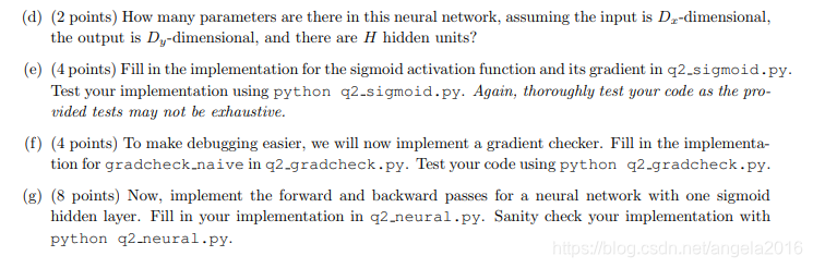
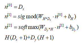
(d)在上圖的神經網路中有多少個引數,假定輸入有Dx維,輸出有Dy維,有H個神經元。
(e)編寫sigmod啟用函式和其梯度的程式
(f)編寫梯度檢測的程式
(g)編寫只有一個sigmod隱藏層的神經網路的前向和後向推導。
解答這幾個問題:
(a)sigmod函式求導

(b) 輸出層的求導情況

(c)主要考的就是鏈式法則的應用,在這個問題中,主要注意的是矩陣的維度的問題,就是到底用不用轉置,需要根據具體的維度變化來決定。

(d)考慮引數的個數,第一層(隱藏層)+第二層(輸出層)
(e) 編寫sigmod函式及其求導函式
#!/usr/bin/env python

import numpy as np


def sigmoid(x):
    """
    Compute the sigmoid function for the input here.

    Arguments:
    x -- A scalar or numpy array.

    Return:
    s -- sigmoid(x)
    """
    s = 1 / (1 + np.exp(-x))
    return s


def sigmoid_grad(s):
    """
    Compute the gradient for the sigmoid function here. Note that
    for this implementation, the input s should be the sigmoid
    function value of your original input x.

    Arguments:
    s -- A scalar or numpy array.

    Return:
    ds -- Your computed gradient.
    """
    ds = s * (1 - s)

    return ds


def test_sigmoid_basic():
    """
    Some simple tests to get you started.
    Warning: these are not exhaustive.
    """
    print "Running basic tests..."
    x = np.array([[1, 2], [-1, -2]])
    f = sigmoid(x)
    g = sigmoid_grad(f)
    print f
    f_ans = np.array([
        [0.73105858, 0.88079708],
        [0.26894142, 0.11920292]])
    assert np.allclose(f, f_ans, rtol=1e-05, atol=1e-06)
    print g
    g_ans = np.array([
        [0.19661193, 0.10499359],
        [0.19661193, 0.10499359]])
    assert np.allclose(g, g_ans, rtol=1e-05, atol=1e-06)
    print "You should verify these results by hand!\n"


if __name__ == "__main__":
    test_sigmoid_basic()
測試結果:

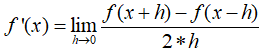
(f) 梯度檢查,利用雙邊檢查,得到的精確度更高。
#!/usr/bin/env python

import numpy as np
import random

# First implement a gradient checker by filling in the following functions
def gradcheck_naive(f, x):
    """ Gradient check for a function f.

    Arguments:
    f -- a function that takes a single argument and outputs the
         cost and its gradients
    x -- the point (numpy array) to check the gradient at
    """

    rndstate = random.getstate()
    random.setstate(rndstate)
    fx, grad = f(x)  # Evaluate function value at original point
    h = 1e-4         # Do not change this!

    # Iterate over all indexes ix in x to check the gradient.
    it = np.nditer(x, flags=['multi_index'], op_flags=['readwrite'])
    while not it.finished:
        ix = it.multi_index

        # Try modifying x[ix] with h defined above to compute numerical
        # gradients (numgrad).

        # Use the centered difference of the gradient.
        # It has smaller asymptotic error than forward / backward difference
        # methods. If you are curious, check out here:
        # https://math.stackexchange.com/questions/2326181/when-to-use-forward-or-central-difference-approximations

        # Make sure you call random.setstate(rndstate)
        # before calling f(x) each time. This will make it possible
        # to test cost functions with built in randomness later.
        x[ix] += h
        f1 = f(x)[0]
        x[ix] -= 2 * h
        f2 = f(x)[0]
        x[ix] += h
        numgrad = (f1-f2)/(2*h)

        # Compare gradients
        reldiff = abs(numgrad - grad[ix]) / max(1, abs(numgrad), abs(grad[ix]))
        if reldiff > 1e-5:
            print "Gradient check failed."
            print "First gradient error found at index %s" % str(ix)
            print "Your gradient: %f \t Numerical gradient: %f" % (
                grad[ix], numgrad)
            return

        it.iternext() # Step to next dimension

    print "Gradient check passed!"

def sanity_check():
    """
    Some basic sanity checks.
    """
    quad = lambda x: (np.sum(x ** 2), x * 2)

    print "Running sanity checks..."
    gradcheck_naive(quad, np.array(123.456))      # scalar test
    gradcheck_naive(quad, np.random.randn(3,))    # 1-D test
    gradcheck_naive(quad, np.random.randn(4,5))   # 2-D test
    print ""

if __name__ == "__main__":
    sanity_check()
程式解釋:在函式gradcheck_naive(f, x) , 其中f是一個函式,接受一個引數的函式,返回的是一個元祖,包含二項,第一項為損失函式cost的數值,第二項為梯度數值;x為進行檢測的輸入的數值,可以是標量,也可以是矩陣(向量)。設定了一個隨機種子,以便你的測試是同一的隨機種子產生,產生正確的結果。然後np.nditer就是一個迭代器,多重索引的迭代器,然後基於索引的基礎上,然後進行雙邊的梯度檢查,然後換下一個資料進行迭代。
【只有實踐,才能發現原來有含糊的地方,是一定會出錯的,不過早出錯比較好。】
在這個地方:我有一個小bug的出現,在這個單個測試中,輸入只是一個數值的情況下,這種方法是適用的,但如果是多個的情況下,f(x[ix]+h)是會出錯的,因為這個時候輸入的是一個數值,而不是整個資料。

(g) 最後一個是實現二層的神經網路(其中一層為隱藏層,一層為輸出層)
#!/usr/bin/env python

import numpy as np
import random

from q1_softmax import softmax
from q2_sigmoid import sigmoid, sigmoid_grad
from q2_gradcheck import gradcheck_naive

def forward_backward_prop(X, labels, params, dimensions):
    """
    Forward and backward propagation for a two-layer sigmoidal network

    Compute the forward propagation and for the cross entropy cost,
    the backward propagation for the gradients for all parameters.

    Notice the gradients computed here are different from the gradients in
    the assignment sheet: they are w.r.t. weights, not inputs.

    Arguments:
    X -- M x Dx matrix, where each row is a training example x.
    labels -- M x Dy matrix, where each row is a one-hot vector.
    params -- Model parameters, these are unpacked for you.
    dimensions -- A tuple of input dimension, number of hidden units
                  and output dimension
    """

    ### Unpack network parameters (do not modify)
    ofs = 0
    Dx, H, Dy = (dimensions[0], dimensions[1], dimensions[2])

    W1 = np.reshape(params[ofs:ofs + Dx * H], (Dx, H))
    ofs += Dx * H
    b1 = np.reshape(params[ofs:ofs + H], (1, H))
    ofs += H
    W2 = np.reshape(params[ofs:ofs + H * Dy], (H, Dy))
    ofs += H * Dy
    b2 = np.reshape(params[ofs:ofs + Dy], (1, Dy))

    # Note: compute cost based on `sum` not `mean`.
    z1 = X.dot(W1) + b1
    a1 = sigmoid(z1)
    z2 = a1.dot(W2) + b2
    a2 = softmax(z2)
    cost = -np.sum(labels * np.log(a2))

    gradz2 = (a2 - labels)
    gradW2 = a1.T.dot(gradz2)
    gradb2 = np.sum(gradz2, axis=0, keepdims=True)
    grada1 = gradz2.dot(W2.T)
    gradz1 = grada1*sigmoid_grad(a1)
    gradW1 = X.T.dot(gradz1)
    gradb1 = np.sum(gradz1, axis=0, keepdims=True)


    ### Stack gradients (do not modify)
    grad = np.concatenate((gradW1.flatten(), gradb1.flatten(), gradW2.flatten(), gradb2.flatten()))
    grad.resize((len(grad), 1))

    return cost, grad

def sanity_check():
    """
    Set up fake data and parameters for the neural network, and test using
    gradcheck.
    """
    print "Running sanity check..."

    N = 20
    dimensions = [10, 5, 10]
    data = np.random.randn(N, dimensions[0])   # each row will be a datum
    labels = np.zeros((N, dimensions[2]))
    for i in xrange(N):
        labels[i, random.randint(0, dimensions[2]-1)] = 1

    params = np.random.randn((dimensions[0] + 1) * dimensions[1] + (
        dimensions[1] + 1) * dimensions[2], 1)

    gradcheck_naive(lambda params: forward_backward_prop(data, labels, params, dimensions), params)


if __name__ == "__main__":
    sanity_check()
在這個問題的實現中,我也犯了一個蠢,就是對於sigmod的求導的地方有含糊,就是不知道到底是那個進行變化,我現在對其重新確定一下。
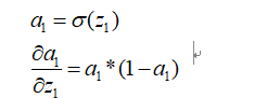
然後在本程式中,呼叫sigmod_grad(a1)就是求上面的這個倒數值。
測試結果:


題目解釋:
(a) 中心詞的索引為c,預測索引為o的詞是否為中心詞的視窗範圍的詞,其中u(w)為字典中的所有的詞的詞向量,其實就是用二套詞向量來進行表示,方便解耦合,簡化學習過程。說了這麼多,這個題目就是求一個梯度。
(b)仍然求一個梯度。
(c)在(a)與(b)中,採用的傳統的,也就是初步的word2vec來實現的,但我們知道採用負取樣的方法,實現效率更高。所以,這個題目就是用來驗證這個結論。用CE loss的執行時間除以negative sampling loss的執行時間來作為speed-up ratio。
(d)word2vec中有二種類別,一種為CBOW, 另一種為skip-gram。視窗大小為m, 然後二種方式的梯度的推導。這是一個不斷擴充套件的問題,一步步的從抽象的情況,擴充套件到具體的情況。
(e)補充word2vec模型,然後利用隨機梯度下降來訓練你自己的詞向量。在檔案中,需要書寫的有:一個歸一化矩陣的行的函式,填充softmax函式和梯度下降函式,補充skip-gram的損失函式和梯度下降函式。(其實就是實現skip-gram)
(f)實現隨機梯度下降演算法
(g)下載實際生活的資料,然後利用補充的程式來訓練詞向量。使用的是斯坦福的語義分析樹語料庫來訓練,這個訓練好的部分會用於下一個部分的語義分析任務。
(h)擴充套件補充CBOW演算法。
題目解答:
(a)(b)(這個地方涉及到了矩陣微分的知識,這個地方的求導有些許的問題,待我看完矩陣微分方法之後來解決這個BUG)

(c)word2vec的負取樣實現中,一次迭代中只需要計算的是K+1個數據, 而對於傳統的softmax方式中,則需要計算的是W+1個數據,所以,時間花費大約為(W+1)/(K+1)

(d)對於skip-gram而言, 推導如下:
現在我們考慮的是一個具體的情況,然後更新的就是vc,對於vj而言,是不做處理的,所以就是視窗範圍內的更新引數。

對於CBOW而言,推導如下:

對於skip-gram而言,簡單說:就是已知中心詞,然後求視窗上下文的情況;對於CBOW而言,簡單說:就是知道視窗上下文的情況,然後求中心詞的情況,中心詞采用上下文次的平均來計算。這樣就可以知道,損失函式到底與什麼有關,與什麼無關了。
(e)這一部分卡了好久,尤其在負取樣那個函式裡面,卡了真的好久好久。雖然難產,但還是產出來了。
在這個程式中,第一個函式NormalizeRows(x)是對輸入資料進行歸一化操作,歸一化的方法是通過按行的模長的歸一化方法。也就是每一行的每一個數值除以此行的向量的模長來實現。(根據給出的例子,也就是test_normalize_rows我們可以推斷出來。)
對於softmaxCostAndGradient函式,就是通過(a)(b)的公式來實現。但一定注意的是矩陣的維度,尤其是對於(3L, )這個問題,很容易出現各種莫名其妙的問題,所以最好就把矩陣的維度統一,這樣比較容易求。
對於getNegativeSamples函式,就是通過隨機取樣函式,來得到K個負取樣的單詞的索引。
對於negSamplingCostAndGradient函式,就是通過(c)的公式來是實現,也是要注意矩陣維度的變化。
對於skipgram(cbow)函式,就是通過(d)的公式,來把每一箇中心詞,上下文詞串起來,最後得到結果。
對於word2vec_sgd_wrapper函式,類似與一個框架,將Word2vecmodel全部框起來,也就是可以採用skipgram實現,也可以採用cbow來實現。
對於test_word2vec函式,就是測試的介面。
#!/usr/bin/env python
# -*- coding:utf-8 -*-

import numpy as np
import random

from q1_softmax import softmax
from q2_gradcheck import gradcheck_naive
from q2_sigmoid import sigmoid, sigmoid_grad

def normalizeRows(x):
    """ Row normalization function
    # 除以模長的歸一化方法
    Implement a function that normalizes each row of a matrix to have
    unit length.
    """

    x = x / (np.sqrt(np.sum(x*x, axis=1, keepdims=True)))
    return x


def test_normalize_rows():
    print "Testing normalizeRows..."
    x = normalizeRows(np.array([[3.0,4.0],[1, 2]]))
    print x
    ans = np.array([[0.6,0.8],[0.4472136,0.89442719]])
    assert np.allclose(x, ans, rtol=1e-05, atol=1e-06)
    print ""


def softmaxCostAndGradient(predicted, target, outputVectors, dataset):
    """ Softmax cost function for word2vec models

    Implement the cost and gradients for one predicted word vector
    and one target word vector as a building block for word2vec
    models, assuming the softmax prediction function and cross
    entropy loss.

    Arguments:
    predicted -- numpy ndarray, predicted word vector (\hat{v} in
                 the written component)
    target -- integer, the index of the target word
    outputVectors -- "output" vectors (as rows) for all tokens
    dataset -- needed for negative sampling, unused here.

    Return:
    cost -- cross entropy cost for the softmax word prediction
    gradPred -- the gradient with respect to the predicted word
           vector
    grad -- the gradient with respect to all the other word
           vectors

    We will not provide starter code for this function, but feel
    free to reference the code you previously wrote for this
    assignment!
    """
    # 為了避免出錯,最好利用reshape來將矩陣來轉變為自己需要的那一種型別, 因為softmax是對行來進行
    predicted = predicted.reshape([1, predicted.shape[0]])
    y_hot = softmax(predicted.dot(outputVectors.T)).reshape([outputVectors.shape[0], 1])
    y_real = np.zeros_like(y_hot)
    y_real[target] = 1
    cost = -np.log(y_hot[target])
    gradPred = (y_hot-y_real).T.dot(outputVectors)
    grad = (y_hot-y_real).dot(predicted)
    return cost, gradPred, grad


def getNegativeSamples(target, dataset, K):

    """ Samples K indexes which are not the target
    隨機負取樣K個數值
    """

    indices = [None] * K
    for k in xrange(K):
        newidx = dataset.sampleTokenIdx()
        while newidx == target:
            newidx = dataset.sampleTokenIdx()
        indices[k] = newidx
    return indices


def negSamplingCostAndGradient(predicted, target, outputVectors, dataset,
                               K=10):
    """ Negative sampling cost function for word2vec models

    Implement the cost and gradients for one predicted word vector
    and one target word vector as a building block for word2vec
    models, using the negative sampling technique. K is the sample
    size.

    Note: See test_word2vec below for dataset's initialization.

    Arguments/Return Specifications: same as softmaxCostAndGradient
    """

    # Sampling of indices is done for you. Do not modify this if you
    # wish to match the autograder and receive points!


    indices = [target]
    indices.extend(getNegativeSamples(target, dataset, K))

    predicted = predicted.reshape([predicted.shape[0], 1])
    gradPred = np.zeros(predicted.shape)
    cost = 0

    soft_vc = sigmoid(outputVectors[target, :].dot(predicted))  # [1, D]*[D, 1]=[1, 1]
    cost -= np.log(soft_vc)
    gradPred += (soft_vc-1.0) * outputVectors[target, :].reshape(predicted.shape)  # [D,1]
    grad_temp = np.zeros([outputVectors.shape[0], 1])    # [M, 1]
    grad_temp[target] = soft_vc-1.0
    for i in range(1, len(indices)):
        soft_vk = sigmoid(-outputVectors[indices[i], :].dot(predicted))
        cost -= np.log(soft_vk)
        gradPred -= (soft_vk-1.0) * outputVectors[indices[i], :].reshape(predicted.shape)
        grad_temp[indices[i]] -= (soft_vk-1.0)
    grad = grad_temp.dot(predicted.T)   # [M, 1]*[1, D]=[M, D]

    return cost, gradPred, grad

def skipgram(currentWord, C, contextWords, tokens, inputVectors, outputVectors,
             dataset, word2vecCostAndGradient=softmaxCostAndGradient):
    """ Skip-gram model in word2vec

    Implement the skip-gram model in this function.

    Arguments:
    currentWord -- a string of the current center word
    C -- integer, context size
    contextWords -- list of no more than 2*C strings, the context words
    tokens -- a dictionary that maps words to their indices in
              the word vector list
    inputVectors -- "input" word vectors (as rows) for all tokens
    outputVectors -- "output" word vectors (as rows) for all tokens
    word2vecCostAndGradient -- the cost and gradient function for
                               a prediction vector given the target
                               word vectors, could be one of the two
                               cost functions you implemented above.

    Return:
    cost -- the cost function value for the skip-gram model
    grad -- the gradient with respect to the word vectors
    """

    cost = 0.0
    gradIn = np.zeros(inputVectors.shape)
    gradOut = np.zeros(outputVectors.shape)

    for word in contextWords:
        cost_1, gradPred1, grad1 = word2vecCostAndGradient(inputVectors[tokens[currentWord]], tokens[word],
                                                              outputVectors, dataset)
        cost += cost_1
        gradIn[tokens[currentWord], :] += np.squeeze([gradPred1])
        gradOut += grad1

    return cost, gradIn, gradOut


def cbow(currentWord, C, contextWords, tokens, inputVectors, outputVectors,
         dataset, word2vecCostAndGradient=softmaxCostAndGradient):
    """CBOW model in word2vec

    Implement the continuous bag-of-words model in this function.

    Arguments/Return specifications: same as the skip-gram model

    Extra credit: Implementing CBOW is optional, but the gradient
    derivations are not. If you decide not to implement CBOW, remove
    the NotImplementedError.
    """

    cost = 0.0
    gradIn = np.zeros(inputVectors.shape)
    gradOut = np.zeros(outputVectors.shape)

    ### YOUR CODE HERE
    raise NotImplementedError
    ### END YOUR CODE

    return cost, gradIn, gradOut


#############################################
# Testing functions below. DO NOT MODIFY!   #
#############################################

def word2vec_sgd_wrapper(word2vecModel, tokens, wordVectors, dataset, C,
                         word2vecCostAndGradient=softmaxCostAndGradient):
    batchsize = 50
    cost = 0.0
    grad = np.zeros(wordVectors.shape)
    N = wordVectors.shape[0]
    inputVectors = wordVectors[:N/2,:]
    outputVectors = wordVectors[N/2:,:]
    for i in xrange(batchsize):
        C1 = random.randint(1,C)
        centerword, context = dataset.getRandomContext(C1)
        if word2vecModel == skipgram:
            denom = 1
        else:
            denom = 1
        c, gin, gout = word2vecModel(
            centerword, C1, context, tokens, inputVectors, outputVectors,
            dataset, word2vecCostAndGradient)
        cost += c / batchsize / denom
        grad[:N/2, :] += gin / batchsize / denom
        grad[N/2:, :] += gout / batchsize / denom

    return cost, grad


def test_word2vec():
    """ Interface to the dataset for negative sampling """
    dataset = type('dummy', (), {})()
    def dummySampleTokenIdx():
        return random.randint(0, 4)

    def getRandomContext(C):
        tokens = ["a", "b", "c", "d", "e"]
        return tokens[random.randint(0,4)], \
            [tokens[random.randint(0,4)] for i in xrange(2*C)]
    dataset.sampleTokenIdx = dummySampleTokenIdx
    dataset.getRandomContext = getRandomContext

    random.seed(31415)
    np.random.seed(9265)
    dummy_vectors = normalizeRows(np.random.randn(10,3))
    dummy_tokens = dict([("a",0), ("b",1), ("c",2),("d",3),("e",4)])
    print "==== Gradient check for skip-gram ===="
    gradcheck_naive(lambda vec: word2vec_sgd_wrapper(
        skipgram, dummy_tokens, vec, dataset, 5, softmaxCostAndGradient),
        dummy_vectors)
    gradcheck_naive(lambda vec: word2vec_sgd_wrapper(
        skipgram, dummy_tokens, vec, dataset, 5, negSamplingCostAndGradient),
        dummy_vectors)
    # print "\n==== Gradient check for CBOW      ===="
    # gradcheck_naive(lambda vec: word2vec_sgd_wrapper(
    #     cbow, dummy_tokens, vec, dataset, 5, softmaxCostAndGradient),
    #     dummy_vectors)
    # gradcheck_naive(lambda vec: word2vec_sgd_wrapper(
    #     cbow, dummy_tokens, vec, dataset, 5, negSamplingCostAndGradient),
    #     dummy_vectors)

    print "\n=== Results ==="
    print skipgram("c", 3, ["a", "b", "e", "d", "b", "c"],
        dummy_tokens, dummy_vectors[:5,:], dummy_vectors[5:,:], dataset)
    print skipgram("c", 1, ["a", "b"],
        dummy_tokens, dummy_vectors[:5,:], dummy_vectors[5:,:], dataset,
        negSamplingCostAndGradient)
    # print cbow("a", 2, ["a", "b", "c", "a"],
    #     dummy_tokens, dummy_vectors[:5,:], dummy_vectors[5:,:], dataset)
    # print cbow("a", 2, ["a", "b", "a", "c"],
    #     dummy_tokens, dummy_vectors[:5,:], dummy_vectors[5:,:], dataset,
    #     negSamplingCostAndGradient)


if __name__ == "__main__":
    test_normalize_rows()
    test_word2vec()
(f)這個是實現SGD函式,這一個填寫的部分比較簡單。
拿到一個這樣需要補全的程式,第一步首先需要明確自己需要補全的那部分程式是那部分了,第二步,if __name__=='__main__'看起,因為這個是程式的入口,然後根據程式的流程來理解。
對於sanity_check函式,就是呼叫sgd的一個介面。
對於sgd函式,引數的每個的意思都在下面。然後在迭代過程中,我們需要通過梯度來更新變數,尤其注意,不要忘記postprocessing函式,因為是一個迭代的過程,不能只在初始的時候對變數進行預處理(歸一化),在迭代過程,也不能忘記呀。
對於save_params函式,就是每隔多少次的迭代,就儲存一下引數的作用。
對於load_saved_params函式,就是匯入之前儲存的引數。
#!/usr/bin/env python

# Save parameters every a few SGD iterations as fail-safe
SAVE_PARAMS_EVERY = 5000

import glob
import random
import numpy as np
import os.path as op
import cPickle as pickle


def load_saved_params():
    """
    A helper function that loads previously saved parameters and resets
    iteration start.
    """
    st = 0
    for f in glob.glob("saved_params_*.npy"):
        iter = int(op.splitext(op.basename(f))[0].split("_")[2])
        if (iter > st):
            st = iter

    if st > 0:
        with open("saved_params_%d.npy" % st, "r") as f:
            params = pickle.load(f)
            state = pickle.load(f)
        return st, params, state
    else:
        return st, None, None


def save_params(iter, params):
    with open("saved_params_%d.npy" % iter, "w") as f:
        pickle.dump(params, f)
        pickle.dump(random.getstate(), f)


def sgd(f, x0, step, iterations, postprocessing=None, useSaved=False,
        PRINT_EVERY=10):
    """ Stochastic Gradient Descent

    Implement the stochastic gradient descent method in this function.

    Arguments:
    f -- the function to optimize, it should take a single
         argument and yield two outputs, a cost and the gradient
         with respect to the arguments
    x0 -- the initial point to start SGD from
    step -- the step size for SGD
    iterations -- total iterations to run SGD for
    postprocessing -- postprocessing function for the parameters
                      if necessary. In the case of word2vec we will need to
                      normalize the word vectors to have unit length.
    PRINT_EVERY -- specifies how many iterations to output loss

    Return:
    x -- the parameter value after SGD finishes
    """

    # Anneal learning rate every several iterations
    ANNEAL_EVERY = 20000

    if useSaved:
        start_iter, oldx, state = load_saved_params()
        if start_iter > 0:
            x0 = oldx
            step *= 0.5 ** (start_iter / ANNEAL_EVERY)

        if state:
            random.setstate(state)
    else:
        start_iter = 0

    x = x0

    if not postprocessing:
        postprocessing = lambda x: x

    expcost = None

    for iter in xrange(start_iter + 1, iterations + 1):
        # Don't forget to apply the postprocessing after every iteration!
        # You might want to print the progress every few iterations.

        cost = None
        ### YOUR CODE HERE
        cost, grad = f(x)
        x -= step * grad
        postprocessing(x)
        ### END YOUR CODE

        if iter % PRINT_EVERY == 0:
            if not expcost:
                expcost = cost
            else:
                expcost = .95 * expcost + .05 * cost
            print "iter %d: %f" % (iter, expcost)

        if iter % SAVE_PARAMS_EVERY == 0 and useSaved:
            save_params(iter, x)

        if iter % ANNEAL_EVERY == 0:
            step *= 0.5

    return x


def sanity_check():
    quad = lambda x: (np.sum(x ** 2), x * 2)

    print "Running sanity checks..."
    t1 = sgd(quad, 0.5, 0.01, 1000, PRINT_EVERY=100)
    print "test 1 result:", t1
    assert abs(t1) <= 1e-6

    t2 = sgd(quad, 0.0, 0.01, 1000, PRINT_EVERY=100)
    print "test 2 result:", t2
    assert abs(t2) <= 1e-6

    t3 = sgd(quad, -1.5, 0.01, 1000, PRINT_EVERY=100)
    print "test 3 result:", t3
    assert abs(t3) <= 1e-6

    print ""


if __name__ == "__main__":
    sanity_check()
(g) 訓練一個語料庫,程式碼如下。
資料集採用的是斯坦福語義分析的資料集。詞向量的維度為10,單詞上下文窗戶大小為5,WordVectors包含二個部分的向量,也就是我們常說的u,v的情況。外層是sgd函式,然後利用sgd的函式應用到word2vec_sgd_warpper上。
迭代40000次,,真的好花費時間呀。
然後對得到的詞向量的情況,對其中的某些單詞進行降維,來看最後的情況單詞的情況。
#!/usr/bin/env python

import random
import numpy as np
from utils.treebank import StanfordSentiment
import matplotlib
matplotlib.use('agg')
import matplotlib.pyplot as plt
import time

from q3_word2vec import *
from q3_sgd import *

# Reset the random seed to make sure that everyone gets the same results
random.seed(314)
dataset = StanfordSentiment()
tokens = dataset.tokens()
nWords = len(tokens)

# We are going to train 10-dimensional vectors for this assignment
dimVectors = 10

# Context size
C = 5

# Reset the random seed to make sure that everyone gets the same results
random.seed(31415)
np.random.seed(9265)

startTime=time.time()
wordVectors = np.concatenate(
    ((np.random.rand(nWords, dimVectors) - 0.5) /
       dimVectors, np.zeros((nWords, dimVectors))),
    axis=0)
wordVectors = sgd(
    lambda vec: word2vec_sgd_wrapper(skipgram, tokens, vec, dataset, C,
        negSamplingCostAndGradient),
    wordVectors, 0.3, 40000, None, True, PRINT_EVERY=10)
# Note that normalization is not called here. This is not a bug,
# normalizing during training loses the notion of length.

print "sanity check: cost at convergence should be around or below 10"
print "training took %d seconds" % (time.time() - startTime)

# concatenate the input and output word vectors
wordVectors = np.concatenate(
    (wordVectors[:nWords,:], wordVectors[nWords:,:]),
    axis=0)
# wordVectors = wordVectors[:nWords,:] + wordVectors[nWords:,:]

visualizeWords = [
    "the", "a", "an", ",", ".", "?", "!", "``", "''", "--",
    "good", "great", "cool", "brilliant", "wonderful", "well", "amazing",
    "worth", "sweet", "enjoyable", "boring", "bad", "waste", "dumb",
    "annoying"]

visualizeIdx = [tokens[word] for word in visualizeWords]
visualizeVecs = wordVectors[visualizeIdx, :]
temp = (visualizeVecs - np.mean(visualizeVecs, axis=0))
covariance = 1.0 / len(visualizeIdx) * temp.T.dot(temp)
U,S,V = np.linalg.svd(covariance)
coord = temp.dot(U[:,0:2])

for i in xrange(len(visualizeWords)):
    plt.text(coord[i,0], coord[i,1], visualizeWords[i],
        bbox=dict(facecolor='green', alpha=0.1))

plt.xlim((np.min(coord[:,0]), np.max(coord[:,0])))
plt.ylim((np.min(coord[:,1]), np.max(coord[:,1])))

plt.savefig('q3_word_vectors.png')
畫出的單詞的影象如下:


題目解釋:使用已經訓練好的詞向量,然後進行一個語義情感分析的步驟,對於語料庫中的每個句子,我們採用單詞的平均詞向量來作為句子的特徵,然後預測句子的情感分析。分為了5個等級,訓練一個softmax分類器來實現目的。
很負面(0),負面(1),中立(2), 積極(3),很積極(4)(a)完成句子向量特徵的計算。利用句子中的詞向量的平均來表示。
(b)解釋為什麼需要在分類時進行正則化。(normalization, regulariza就tion)
(c)填寫超引數選擇的程式碼來尋找最好的超引數。至少要在驗證集和測試集上達到36.5%的準確率。
(d)使用自己訓練的詞向量來跑情感分類的程式,然後使用已經訓練好的GLOVE模型來跑情感分類的程式,比較在訓練集,驗證集和測試集上的準確率。為什麼預訓練的GLOVE模型效果更好,明確並提出至少3個不同的原因。
(e)畫出使用GLOVE詞向量的訓練集合驗證集上的準確率曲線,採用log函式來做處理。剪短的解釋從曲線中得到什麼。
(f)分析模型產生錯誤的原因,簡短的解釋混淆矩陣。
(g)分析3個分類錯誤的例子來進行解釋,並且簡短的說明什麼樣的特徵總能夠將會被分類錯誤。盡力的找出錯誤的原因。
題目解答:
(a)就是利用句子的每個單詞的詞向量的平均來作為句子的特徵,來進行處理。具體程式在後面。
但自己寫的程式效率不是特別高,因為沒有很好的利用到向量化的手段,需要不斷的進行學習。
(b)正則化的好壞就在於防止過擬合。正則化的常用的方法為L1正則化,L2正則化。對於L2正則化而言,減少引數的數值,以便在資料發生偏移的時候,結果影響不大,也就是提高模型對於未知例項的泛化能力。
(c)在getRegularizarionValues函式中,通過函式來給values賦一系列的浮點數的值。
在chooseBestModel函式中,通過字典中的關鍵字dev來進行排序。
(d)結果顯示:
對於youevectors而言:
=== Recap ===
Reg             Train   Dev     Test
1.00E-02        30.946  32.334  29.910
1.10E-02        30.922  32.334  29.955
1.20E-02        30.946  32.334  29.910
1.32E-02        30.922  32.243  29.955
1.45E-02        30.840  32.153  30.000
1.59E-02        30.770  32.153  30.000
1.75E-02        30.735  32.243  29.910
1.92E-02        30.817  31.789  29.955
2.10E-02        30.735  31.698  29.955
2.31E-02        30.770  31.698  29.955
2.54E-02        30.618  31.608  30.000
2.78E-02        30.501  31.608  30.090
3.05E-02        30.524  31.698  29.910
3.35E-02        30.431  31.608  29.955
3.68E-02        30.360  31.698  29.819
4.04E-02        30.325  31.608  29.864
4.43E-02        30.302  31.880  30.045
4.86E-02        30.349  31.880  30.136
5.34E-02        30.384  31.971  29.955
5.86E-02        30.396  32.062  29.955
6.43E-02        30.349  32.153  30.000
7.05E-02        30.372  32.243  30.045
7.74E-02        30.325  32.425  30.045
8.50E-02        30.290  32.062  30.136
9.33E-02        30.302  31.880  29.955
1.02E-01        30.302  31.971  29.910
1.12E-01        30.314  31.789  29.729
1.23E-01        30.279  31.971  29.638
1.35E-01        30.185  31.789  29.774
1.48E-01        30.162  31.880  29.638
1.63E-01        30.044  31.789  29.502
1.79E-01        29.998  32.062  29.367
1.96E-01        29.963  31.971  29.412
2.15E-01        29.740  32.062  29.502
2.36E-01        29.635  31.698  29.321
2.60E-01        29.717  31.971  29.095
2.85E-01        29.494  32.062  29.005
3.13E-01        29.459  31.880  28.824
3.43E-01        29.506  31.789  28.778
3.76E-01        29.459  31.517  28.371
4.13E-01        29.424  31.335  28.326
4.53E-01        29.295  31.335  28.281
4.98E-01        29.260  31.244  28.326
5.46E-01        29.377  30.790  28.100
5.99E-01        29.412  31.244  28.054
6.58E-01        29.436  31.153  28.145
7.22E-01        29.389  30.881  28.145
7.92E-01        29.377  30.336  27.873
8.70E-01        29.190  29.973  27.783
9.55E-01        28.968  29.882  27.240
1.05E+00        28.816  29.609  27.059
1.15E+00        28.862  29.064  26.561
1.26E+00        28.663  28.520  26.335
1.38E+00        28.640  28.065  25.928
1.52E+00        28.546  27.520  25.928
1.67E+00        28.500  27.430  25.701
1.83E+00        28.265  27.339  25.339
2.01E+00        27.926  26.794  25.204
2.21E+00        27.938  26.431  24.887
2.42E+00        27.961  26.703  24.615
2.66E+00        27.891  26.703  24.525
2.92E+00        27.680  26.431  24.208
3.20E+00        27.680  26.158  23.846
3.51E+00        27.575  25.704  23.846
3.85E+00        27.551  25.704  23.665
4.23E+00        27.446  25.522  23.620
4.64E+00        27.353  25.522  23.394
5.09E+00        27.353  25.522  23.213
5.59E+00        27.317  25.704  23.122
6.14E+00        27.306  25.704  23.122
6.73E+00        27.271  25.704  23.122
7.39E+00        27.247  25.522  23.122
8.11E+00        27.247  25.522  23.122
8.90E+00        27.235  25.522  23.122
9.77E+00        27.247  25.522  23.077
1.07E+01        27.235  25.522  23.077
1.18E+01        27.235  25.522  23.077
1.29E+01        27.235  25.522  23.077
1.42E+01        27.235  25.522  23.077
1.56E+01        27.235  25.522  23.032
1.71E+01        27.235  25.522  23.032
1.87E+01        27.235  25.522  23.032
2.06E+01        27.235  25.522  23.032
2.26E+01        27.235  25.522  23.032
2.48E+01        27.235  25.522  23.032
2.72E+01        27.235  25.522  23.032
2.98E+01        27.247  25.522  23.032
3.27E+01        27.247  25.522  23.032
3.59E+01        27.247  25.522  23.032
3.94E+01        27.247  25.522  23.032
4.33E+01        27.247  25.522  23.032
4.75E+01        27.247  25.522  23.032
5.21E+01        27.247  25.522  23.032
5.72E+01        27.247  25.522  23.032
6.28E+01        27.247  25.522  23.032
6.89E+01        27.247  25.522  23.032
7.56E+01        27.247  25.522  23.032
8.30E+01        27.247  25.522  23.032
9.11E+01        27.247  25.522  23.032
1.00E+02        27.247  25.522  23.032

Best regularization value: 7.74E-02
Test accuracy (%): 30.045249
對於pretrained而言:
=== Recap ===
Reg             Train   Dev     Test
1.00E-02        39.923  36.331  37.195
1.10E-02        39.934  36.331  37.195
1.20E-02        39.911  36.240  37.195
1.32E-02        39.899  36.240  37.195
1.45E-02        39.899  36.421  37.285
1.59E-02        39.888  36.694  37.285
1.75E-02        39.876  36.603  37.240
1.92E-02        39.841  36.603  37.195
2.10E-02        39.853  36.694  37.285
2.31E-02        39.864  36.421  37.240
2.54E-02        39.864  36.421  37.421
2.78E-02        39.853  36.331  37.285
3.05E-02        39.853  36.421  37.376
3.35E-02        39.876  36.421  37.466
3.68E-02        39.841  36.331  37.511
4.04E-02        39.817  36.331  37.511
4.43E-02        39.829  36.331  37.466
4.86E-02        39.923  36.240  37.511
5.34E-02        39.888  36.240  37.466
5.86E-02        39.853  36.331  37.421
6.43E-02        39.876  36.331  37.330
7.05E-02        39.864  36.331  37.195
7.74E-02        39.864  36.421  37.195
8.50E-02        39.864  36.331  37.240
9.33E-02        39.853  36.331  37.195
1.02E-01        39.817  36.240  37.149
1.12E-01        39.735  36.240  37.195
1.23E-01        39.771  36.512  37.285
1.35E-01        39.735  36.512  37.466
1.48E-01        39.794  36.512  37.511
1.63E-01        39.806  36.512  37.466
1.79E-01        39.841  36.421  37.376
1.96E-01        39.747  36.421  37.330
2.15E-01        39.724  36.512  37.240
2.36E-01        39.665  36.512  37.195
2.60E-01        39.654  36.512  37.195
2.85E-01        39.560  36.421  37.330
3.13E-01        39.583  36.240  37.285
3.43E-01        39.642  36.240  37.285
3.76E-01        39.630  36.331  37.285
4.13E-01        39.630  36.331  37.285
4.53E-01        39.607  36.149  37.330
4.98E-01        39.618  36.149  37.330
5.46E-01        39.583  36.149  37.330
5.99E-01        39.583  36.149  37.285
6.58E-01        39.607  36.421  37.240
7.22E-01        39.548  36.512  37.285
7.92E-01        39.537  36.512  37.285
8.70E-01        39.525  36.603  37.376
9.55E-01        39.525  36.603  37.285
1.05E+00        39.478  36.512  37.330
1.15E+00        39.525  36.603  37.285
1.26E+00        39.537  36.512  37.330
1.38E+00        39.548  36.512  37.330
1.52E+00        39.490  36.512  37.285
1.67E+00        39.490  36.603  37.059
1.83E+00        39.466  36.694  37.195
2.01E+00        39.501  36.876  37.240
2.21E+00        39.431  36.694  37.240
2.42E+00        39.408  36.603  37.240
2.66E+00        39.302  36.876  37.195
2.92E+00        39.279  36.876  37.195
3.20E+00        39.197  36.966  37.104
3.51E+00        39.022  36.876  37.240
3.85E+00        39.115  36.694  37.285
4.23E+00        39.092  36.785  37.376
4.64E+00        39.010  36.876  37.285
5.09E+00        38.963  36.694  37.376
5.59E+00        39.010  36.512  37.466
6.14E+00        38.951  36.785  37.466
6.73E+00        38.928  36.876  37.783
7.39E+00        38.893  36.785  37.828
8.11E+00        38.846  36.694  37.828
8.90E+00        38.729  36.694  37.828
9.77E+00        38.647  36.876  37.738
1.07E+01        38.706  36.876  37.466
1.18E+01        38.659  37.239  37.511
1.29E+01        38.542  37.057  37.421
1.42E+01        38.448  36.876  37.330
1.56E+01        38.343  36.694  37.149
1.71E+01        38.319  36.966  37.240
1.87E+01        38.191  36.694  37.149
2.06E+01        38.191  36.603  37.059
2.26E+01        38.003  36.421  36.968
2.48E+01        37.863  36.331  36.833
2.72E+01        37.746  36.694  36.923
2.98E+01        37.617  36.966  36.697
3.27E+01        37.500  36.876  36.471
3.59E+01        37.512  36.785  36.290
3.94E+01        37.477  36.603  36.425
4.33E+01        37.383  36.512  36.244
4.75E+01        37.161  36.512  36.199
5.21E+01        37.125  36.421  36.290
5.72E+01        36.997  36.149  36.063
6.28E+01        36.821  35.786  36.154
6.89E+01        36.809  35.695  36.018
7.56E+01        36.610  35.876  35.882
8.30E+01        36.575  35.332  35.611
9.11E+01        36.482  34.968  35.656
1.00E+02        36.330  35.059  35.701

Best regularization value: 1.18E+01
Test accuracy (%): 37.511312
對於Glove比自己訓練的詞向量效能更好的原因:
1,因為Glove使用的維度更高,使用的是50維,而我們自己訓練的詞向量是10維。
2,訓練GLove時採用的是很大的語料庫,然後可以得到一個更全面的效果,而我們訓練的語料庫資料量不夠大,不能得到無偏的詞向量。
3,對於Glove而言,使用到了全域性的資訊,使用了詞向量共現的資訊,而對於Word2vec而言,使用的是上下文的區域性關係。
(e)畫出的不同正則化引數的訓練集,驗證集的準確率的情況。(採用Glove訓練的)

這幅圖展現的是不同的正則化係數對於訓練集和驗證集的準確率的影響。對於正則化係數一直增大,對於訓練集的準確率一直在下降,而驗證集資料有一個小範圍的上升的過程,說明起到了避免過擬合訓練資料的效果,而正則化係數太大,二者的準確率都很低,說明模型太簡單了,導致了模型沒有很好的擬合數據。
(f)畫出的混淆矩陣圖形如下:(使用Glove模型)

分析上面的混淆矩陣,在很消極的資料中,很多的被分為了消極,次多被分為了積極;消極的資料中,很多被分為了消極,但也有次多的被分為了積極;在中立的資料彙總,很多被分為了消極,次多被分為了積極;在積極的資料中,很多的被分為積極,少部分被分為了消極;在很積極的資料中,很多被分為了積極,次多的被分為很積極。
在我們構建的這個模型中,對於積極的資料分類效果最好,其次是消極的資料,其次是很積極的資料,中立的資料,最後是很消極的資料。
總體來看,對於積極方面的資料效果更好,對於中立和消極的資料分類效果一般。
(g)分析三條分錯的資料。
資料:
True	Predicted	Text
3	4	it 's a lovely film with lovely performances by buy and accorsi .
2	1	no one goes unindicted here , which is probably for the best .
3	1	and if you 're not nearly moved to tears by a couple of scenes , you 've got ice water in your veins .
對於第一條:
從積極的資料預測為很積極的資料。因為這二者的界限很模糊,不是將明顯的積極的資料分為消極的這類嚴重的錯誤。
對於第二條:
可能否定詞和不確定的詞有點多,所以將其偏向了消極的觀點。
對於第三條:
涉及到了反語,有一些偏消極的詞,沒有學習到反語的意思,出錯。
解釋程式:這個程式的入口程式:main函式,引數為另一個函式getArguments。
首先說,getArguments函式,這個呼叫了argparse包,這個包用於從python內建的一個用於命令項選項與引數解析的模組,通過在程式中定義好需要的引數,然後argparse會幫我們從sys.argv中解析出這些引數,並自動生成幫助和使用資訊。這個是需要在命令列下進行執行的。
具體講解連結:https://www.jianshu.com/p/fef2d215b91d
https://blog.csdn.net/u013177568/article/details/62432761/
我覺得我差一點就陣亡在這個地方,但我最後還是解決了這個問題。在這個地方遇到的問題是我對於那個argparse包的不熟悉,不知道該怎麼執行,具體詳見上面的連結。
還有一個問題,因為我是windows環境,利用命令列的時候要cd到這個資料夾下執行,否則的話會報找不到檔案的錯誤,因為是從系統盤C盤找的,這當然找不到了。
這裡再貼一個連結,https://www.cnblogs.com/wangguoyuan-09/p/6866798.html,講的是pycharm來執行命令列程式。
其次,說的是main函式,資料集採用的是斯坦福情感分析的資料集,然後根據命令列的引數(互斥的),選擇是採用pretrained,還是採用yourvectors;然後讀取到資料集中的訓練集,驗證集和測試集,抽取資料的特徵;然後驗證不同的正則化引數的訓練結果,然後輸出結果。對於pretrained的類別,還會畫出圖來進行錯誤分析。
對於getSentenceFeatures函式,就是(a)中,利用句子的每個單詞的詞向量的平均來作為整個句子的特徵來進行處理。
對於getRegularizationValues函式,就是(b)中,得到一系列的正則化的引數,然後對這些資料進行排序。
對於chooseBestModel函式,就是(b)中,根據驗證集的準確率來選擇一個好的模型。
對於accuracy函式,就是通過向量化的手段,來得到準確率的計算。
對於plotRegVsAccuracy函式,就是通過畫出正則化引數以及準確率的變化的曲線的函式。
對於outputConfusionMatrix是用來畫出混淆矩陣的函式。
在這個地方有比較多的學習的地方:
1)對於混淆矩陣的畫法,不是僅僅得到一個矩陣就OK, 也是可以畫出影象的,很美觀。
2)自己有很多可以借鑑的地方
貼出matplotlib官網的連結以便後續檢視:https://matplotlib.org/api/pyplot_summary.html
對於outputPredictions是用來輸出一個txt文件,裡面記錄了驗證集資料的真實的標籤,預測的標籤,以及資料。
最後的程式實現如下:
#!/usr/bin/env python
# -*- coding:utf-8 -*-

import argparse
import numpy as np
import matplotlib
matplotlib.use('agg')
import matplotlib.pyplot as plt
import itertools

from utils.treebank import StanfordSentiment
import utils.glove as glove

from q3_sgd import load_saved_params, sgd

# We will use sklearn here because it will run faster than implementing
# ourselves. However, for other parts of this assignment you must implement
# the functions yourself!
from sklearn.linear_model import LogisticRegression
from sklearn.metrics import confusion_matrix


def getArguments():
    parser = argparse.ArgumentParser()
    group = parser.add_mutually_exclusive_group(required=True)
    group.add_argument("--pretrained", dest="pretrained", action="store_true",
                       help="Use pretrained GloVe vectors.")
    group.add_argument("--yourvectors", dest="yourvectors", action="store_true",
                       help="Use your vectors from q3.")
    return parser.parse_args()


def getSentenceFeatures(tokens, wordVectors, sentence):
    """
    Obtain the sentence feature for sentiment analysis by averaging its
    word vectors
    """

    # Implement computation for the sentence features given a sentence.

    # Inputs:
    # tokens -- a dictionary that maps words to their indices in
    #           the word vector list
    # wordVectors -- word vectors (each row) for all tokens
    # sentence -- a list of words in the sentence of interest

    # Output:
    # - sentVector: feature vector for the sentence

    sentVector = np.zeros((wordVectors.shape[1],))

    for word in sentence:
        sentVector += wordVectors[tokens[word]]
    sentVector *= 1.0/len(sentence)

    assert sentVector.shape == (wordVectors.shape[1],)
    return sentVector


def getRegularizationValues():
    """Try different regularizations

    Return a sorted list of values to try.
    """
    # Assign a list of floats in the block below
    values = np.logspace(-2, 2, num=100, base=10)
    return sorted(values)


def chooseBestModel(results):
    """Choose the best model based on dev set performance.

    Arguments:
    results -- A list of python dictionaries of the following format:
        {
            "reg": regularization,
            "clf": classifier,
            "train": trainAccuracy,
            "dev": devAccuracy,
            "test": testAccuracy
        }

    Each dictionary represents the performance of one model.

    Returns:
    Your chosen result dictionary.
    """
    # 對於利用dev的關鍵字來進行排序
    bestResult = max(results, key=lambda x: x['dev'])

    return bestResult


def accuracy(y, yhat):
    """ Precision for classifier """
    assert(y.shape == yhat.shape)
    return np.sum(y == yhat) * 100.0 / y.size


def plotRegVsAccuracy(regValues, results, filename):
    """ Make a plot of regularization vs accuracy """
    plt.plot(regValues, [x["train"] for x in results])
    plt.plot(regValues, [x["dev"] for x in results])
    plt.xscale('log')
    plt.xlabel("regularization")
    plt.ylabel("accuracy")
    plt.legend(['train', 'dev'], loc='upper left')
    plt.savefig(filename)


def outputConfusionMatrix(features, labels, clf, filename):
    """ Generate a confusion matrix """
    pred = clf.predict(features)
    cm = confusion_matrix(labels, pred, labels=range(5))
    plt.figure()
    plt.imshow(cm, interpolation='nearest', cmap=plt.cm.Reds)
    plt.colorbar()
    classes = ["- -", "-", "neut", "+", "+ +"]
    tick_marks = np.arange(len(classes))
    plt.xticks(tick_marks, classes)
    plt.yticks(tick_marks, classes)
    thresh = cm.max() / 2.
    for i, j in itertools.product(range(cm.shape[0]), range(cm.shape[1])):
        plt.text(j, i, cm[i, j],
                 horizontalalignment="center",
                 color="white" if cm[i, j] > thresh else "black")
    plt.tight_layout()
    plt.ylabel('True label')
    plt.xlabel('Predicted label')
    plt.savefig(filename)


def outputPredictions(dataset, features, labels, clf, filename):
    """ Write the predictions to file """
    pred = clf.predict(features)
    with open(filename, "w") as f:
        print >> f, "True\tPredicted\tText"
        for i in xrange(len(dataset)):
            print >> f, "%d\t%d\t%s" % (
                labels[i], pred[i], " ".join(dataset[i][0]))


def main(args):
    """ Train a model to do sentiment analyis"""

    # Load the dataset
    dataset = StanfordSentiment()
    tokens = dataset.tokens()
    nWords = len(tokens)

    if args.yourvectors:
        _, wordVectors, _ = load_saved_params()
        wordVectors = np.concatenate(
            (wordVectors[:nWords,:], wordVectors[nWords:,:]),
            axis=1)
    elif args.pretrained:
        wordVectors = glove.loadWordVectors(tokens)
    dimVectors = wordVectors.shape[1]

    # Load the train set
    trainset = dataset.getTrainSentences()
    nTrain = len(trainset)
    trainFeatures = np.zeros((nTrain, dimVectors))
    trainLabels = np.zeros((nTrain,), dtype=np.int32)
    for i in xrange(nTrain):
        words, trainLabels[i] = trainset[i]
        trainFeatures[i, :] = getSentenceFeatures(tokens, wordVectors, words)

    # Prepare dev set features
    devset = dataset.getDevSentences()
    nDev = len(devset)
    devFeatures = np.zeros((nDev, dimVectors))
    devLabels = np.zeros((nDev,), dtype=np.int32)
    for i in xrange(nDev):
        words, devLabels[i] = devset[i]
        devFeatures[i, :] = getSentenceFeatures(tokens, wordVectors, words)

    # Prepare test set features
    testset = dataset.getTestSentences()
    nTest = len(testset)
    testFeatures = np.zeros((nTest, dimVectors))
    testLabels = np.zeros((nTest,), dtype=np.int32)
    for i in xrange(nTest):
        words, testLabels[i] = testset[i]
        testFeatures[i, :] = getSentenceFeatures(tokens, wordVectors, words)

    # We will save our results from each run
    results = []
    regValues = getRegularizationValues()
    for reg in regValues:
        print "Training for reg=%f" % reg
        # Note: add a very small number to regularization to please the library
        clf = LogisticRegression(C=1.0/(reg + 1e-12))
        clf.fit(trainFeatures, trainLabels)

        # Test on train set
        pred = clf.predict(trainFeatures)
        trainAccuracy = accuracy(trainLabels, pred)
        print "Train accuracy (%%): %f" % trainAccuracy

        # Test on dev set
        pred = clf.predict(devFeatures)
        devAccuracy = accuracy(devLabels, pred)
        print "Dev accuracy (%%): %f" % devAccuracy

        # Test on test set
        # Note: always running on test is poor style. Typically, you should
        # do this only after validation.
        pred = clf.predict(testFeatures)
        testAccuracy = accuracy(testLabels, pred)
        print "Test accuracy (%%): %f" % testAccuracy

        results.append({
            "reg": reg,
            "clf": clf,
            "train": trainAccuracy,
            "dev":