We can train this kind of neural network in a few minutes on a modern laptop. When it’s done, we’ll have a neural network that can recognize pictures of “8”s with a pretty high accuracy. Welcome to the world of (late 1980’s-era) image recognition!

Tunnel Vision

It’s really neat that simply feeding pixels into a neural network actually worked to build image recognition! Machine learning is magic! …right?

Well, of course it’s not that simple.

First, the good news is that our “8” recognizer really does work well on simple images where the letter is right in the middle of the image:

But now the really bad news:

Our “8” recognizer totally fails to work when the letter isn’t perfectly centered in the image. Just the slightest position change ruins everything:

This is because our network only learned the pattern of a perfectly-centered “8”. It has absolutely no idea what an off-center “8” is. It knows exactly one pattern and one pattern only.

That’s not very useful in the real world. Real world problems are never that clean and simple. So we need to figure out how to make our neural network work in cases where the “8” isn’t perfectly centered.

Brute Force Idea #1: Searching with a Sliding Window

We already created a really good program for finding an “8” centered in an image. What if we just scan all around the image for possible “8”s in smaller sections, one section at a time, until we find one?

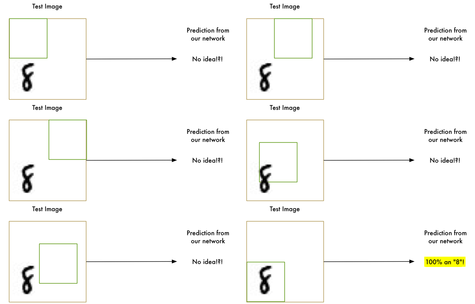
This approach called a sliding window. It’s the brute force solution. It works well in some limited cases, but it’s really inefficient. You have to check the same image over and over looking for objects of different sizes. We can do better than this!

Brute Force Idea #2: More data and a Deep Neural Net

When we trained our network, we only showed it “8”s that were perfectly centered. What if we train it with more data, including “8”s in all different positions and sizes all around the image?

We don’t even need to collect new training data. We can just write a script to generate new images with the “8”s in all kinds of different positions in the image:

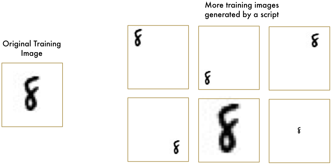
Using this technique, we can easily create an endless supply of training data.

More data makes the problem harder for our neural network to solve, but we can compensate for that by making our network bigger and thus able to learn more complicated patterns.

To make the network bigger, we just stack up layer upon layer of nodes:

We call this a “deep neural network” because it has more layers than a traditional neural network.

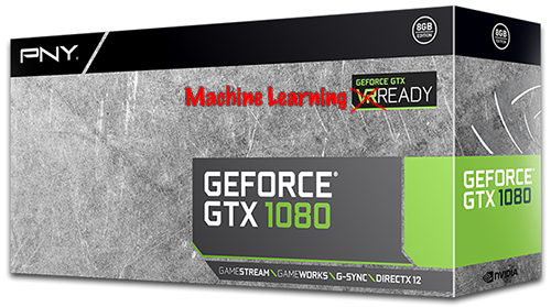
This idea has been around since the late 1960s. But until recently, training this large of a neural network was just too slow to be useful. But once we figured out how to use 3d graphics cards (which were designed to do matrix multiplication really fast) instead of normal computer processors, working with large neural networks suddenly became practical. In fact, the exact same NVIDIA GeForce GTX 1080 video card that you use to play Overwatch can be used to train neural networks incredibly quickly.

But even though we can make our neural network really big and train it quickly with a 3d graphics card, that still isn’t going to get us all the way to a solution. We need to be smarter about how we process images into our neural network.

Think about it. It doesn’t make sense to train a network to recognize an “8” at the top of a picture separately from training it to recognize an “8” at the bottom of a picture as if those were two totally different objects.

There should be some way to make the neural network smart enough to know that an “8” anywhere in the picture is the same thing without all that extra training. Luckily… there is!

The Solution is Convolution

As a human, you intuitively know that pictures have a hierarchy or conceptual structure. Consider this picture:

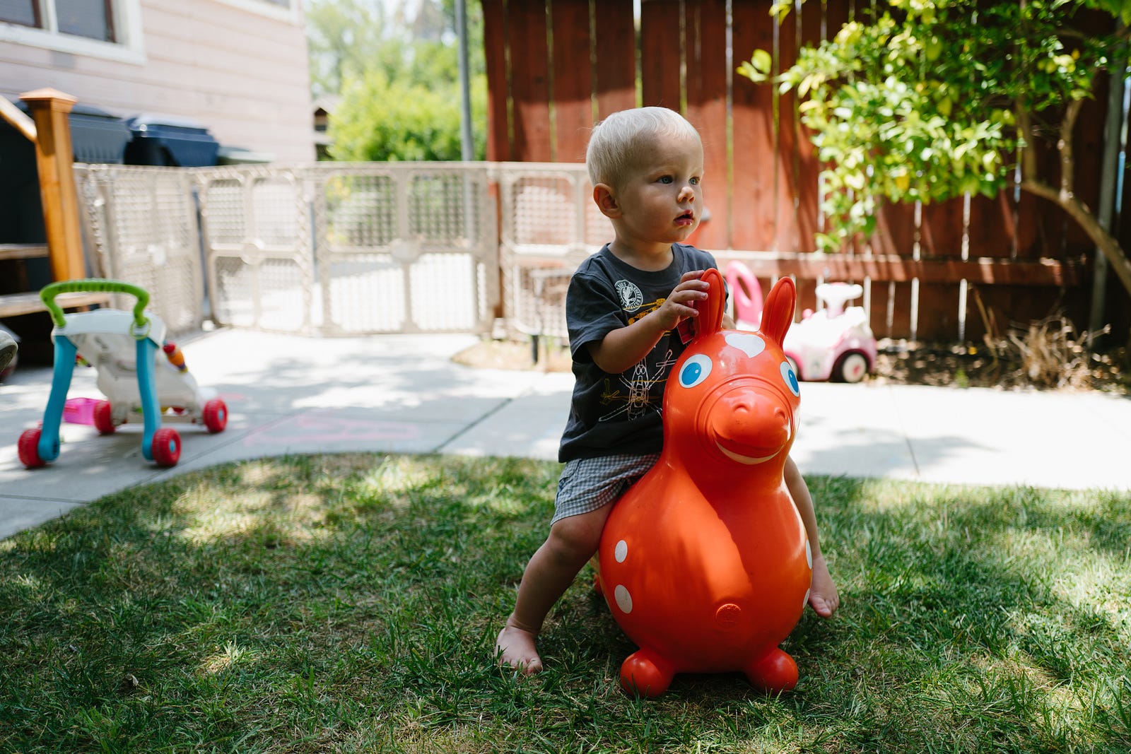
As a human, you instantly recognize the hierarchy in this picture:

• The ground is covered in grass and concrete
• There is a child
• The child is sitting on a bouncy horse
• The bouncy horse is on top of the grass

Most importantly, we recognize the idea of a child no matter what surface the child is on. We don’t have to re-learn the idea of child for every possible surface it could appear on.

But right now, our neural network can’t do this. It thinks that an “8” in a different part of the image is an entirely different thing. It doesn’t understand that moving an object around in the picture doesn’t make it something different. This means it has to re-learn the identify of each object in every possible position. That sucks.

We need to give our neural network understanding of translation invariance — an “8” is an “8” no matter where in the picture it shows up.

We’ll do this using a process called Convolution. The idea of convolution is inspired partly by computer science and partly by biology (i.e. mad scientists literally poking cat brains with weird probes to figure out how cats process images).

How Convolution Works

Instead of feeding entire images into our neural network as one grid of numbers, we’re going to do something a lot smarter that takes advantage of the idea that an object is the same no matter where it appears in a picture.

Here’s how it’s going to work, step by step —

Step 1: Break the image into overlapping image tiles

Similar to our sliding window search above, let’s pass a sliding window over the entire original image and save each result as a separate, tiny picture tile:

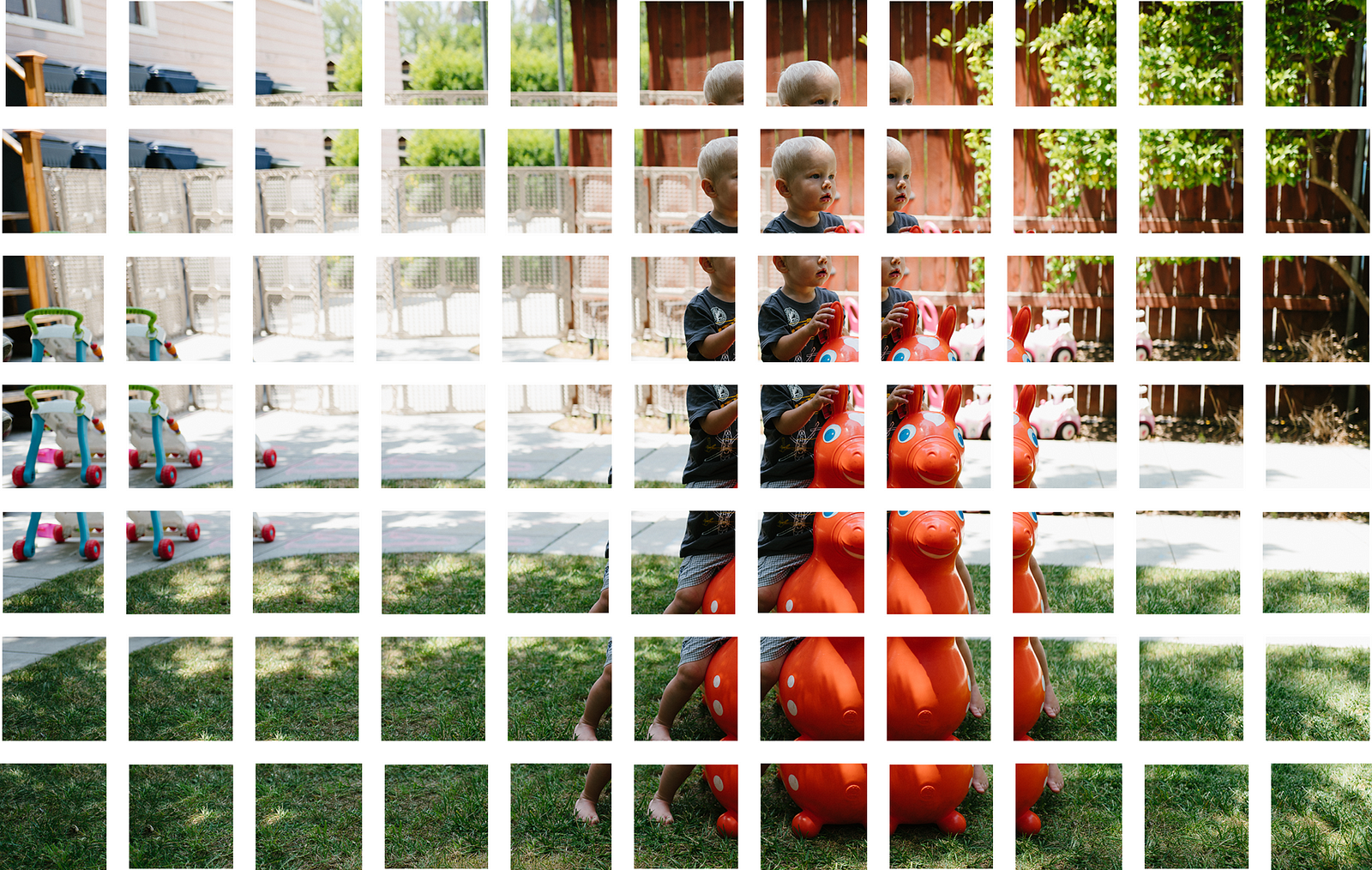
By doing this, we turned our original image into 77 equally-sized tiny image tiles.

Step 2: Feed each image tile into a small neural network

Earlier, we fed a single image into a neural network to see if it was an “8”. We’ll do the exact same thing here, but we’ll do it for each individual image tile:

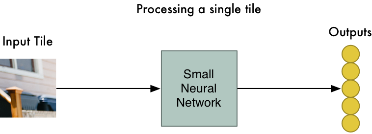
However, there’s one big twist: We’ll keep the same neural network weights for every single tile in the same original image. In other words, we are treating every image tile equally. If something interesting appears in any given tile, we’ll mark that tile as interesting.

Step 3: Save the results from each tile into a new array

We don’t want to lose track of the arrangement of the original tiles. So we save the result from processing each tile into a grid in the same arrangement as the original image. It looks like this:

In other words, we’ve started with a large image and we ended with a slightly smaller array that records which sections of our original image were the most interesting.

Step 4: Downsampling

The result of Step 3 was an array that maps out which parts of the original image are the most interesting. But that array is still pretty big:

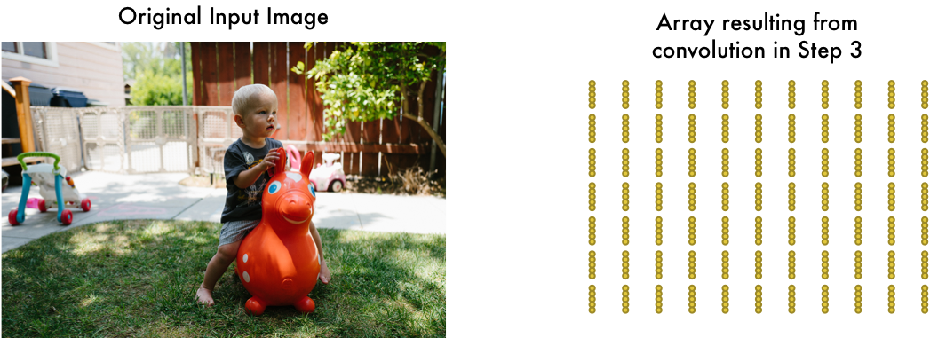
To reduce the size of the array, we downsample it using an algorithm called max pooling. It sounds fancy, but it isn’t at all!

We’ll just look at each 2x2 square of the array and keep the biggest number:

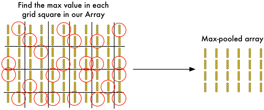
The idea here is that if we found something interesting in any of the four input tiles that makes up each 2x2 grid square, we’ll just keep the most interesting bit. This reduces the size of our array while keeping the most important bits.

Final step: Make a prediction

So far, we’ve reduced a giant image down into a fairly small array.

Guess what? That array is just a bunch of numbers, so we can use that small array as input into another neural network. This final neural network will decide if the image is or isn’t a match. To differentiate it from the convolution step, we call it a “fully connected” network.

So from start to finish, our whole five-step pipeline looks like this:

Adding Even More Steps

Our image processing pipeline is a series of steps: convolution, max-pooling, and finally a fully-connected network.

When solving problems in the real world, these steps can be combined and stacked as many times as you want! You can have two, three or even ten convolution layers. You can throw in max pooling wherever you want to reduce the size of your data.

The basic idea is to start with a large image and continually boil it down, step-by-step, until you finally have a single result. The more convolution steps you have, the more complicated features your network will be able to learn to recognize.

For example, the first convolution step might learn to recognize sharp edges, the second convolution step might recognize beaks using it’s knowledge of sharp edges, the third step might recognize entire birds using it’s knowledge of beaks, etc.

Here’s what a more realistic deep convolutional network (like you would find in a research paper) looks like:

In this case, they start a 224 x 224 pixel image, apply convolution and max pooling twice, apply convolution 3 more times, apply max pooling and then have two fully-connected layers. The end result is that the image is classified into one of 1000 categories!

Constructing the Right Network

So how do you know which steps you need to combine to make your image classifier work?

Honestly, you have to answer this by doing a lot of experimentation and testing. You might have to train 100 networks before you find the optimal structure and parameters for the problem you are solving. Machine learning involves a lot of trial and error!

Building our Bird Classifier

Now finally we know enough to write a program that can decide if a picture is a bird or not.

As always, we need some data to get started. The free CIFAR10 data set contains 6,000 pictures of birds and 52,000 pictures of things that are not birds. But to get even more data we’ll also add in the Caltech-UCSD Birds-200–2011 data set that has another 12,000 bird pics.

Here’s a few of the birds from our combined data set: