Awesome seaborn for Data Visualisation — Part 1

Data visualization is one of the most important parts of in Data Science. It is often said that a picture is worth a thousand words, and this is no different in Data Science. Often times, communicating relationships between variables in Data or other findings can be made easier with Data Visualizations. Many executives do not have time to read long reports or technical writings about machine learning projects. They need visualizations that can tell them all they need to know about data at one glance. This is where data visualization comes in. There are several Data Visualization tools that can help you turn data into insightful pictures. One such is the

What is Seaborn?

Seaborn is a data visualization package for python that is based on the Matplotlib. Seaborn allows Data Scientists to make high-level and interactive visualizations that are better than anything Matplotlib offers. Users can also combine several variables and make visualizations more beautiful than regular Matplotlib.

In this tutorial, we will look at everything about getting started with Seaborn for data visualization. We will first look at how to plot single categorical or numerical variables with Seaborn. Thereafter, we will look at two variables on a single plot, then finally multivariate and 3D plots.

In performing this tutorial, we will be using two datasets:

1. A dataset containing various information about automobile vehicles
2. A dataset containing information about police killings in the United States of America

We will explore the relationship between various variables in both these datasets, all with the aid of the Seaborn package.

The first thing to do is to import the following libraries

• Pandas for data manipulation
• Matplotlib for basic visualization
• Seaborn for improved and interactive visualization

import pandas as pd import seaborn as sns import matplotlib.pyplot as plt %matplotlib inline

The first dataset is a set of vehicle information. The second data set is information about police killings in the United States

#Import the data sets vehicles = pd.read_csv('vehicles.csv') police_killings = pd.read_csv('PoliceKillingsUS.csv', encoding = 'Windows-1252')

#Check the general info of the dataset police_killings.info() vehicles.info()

Below is the execution result:

<class 'pandas.core.frame.DataFrame'>RangeIndex: 2535 entries, 0 to 2534Data columns (total 13 columns):id                         2535 non-null int64name                       2535 non-null objectmanner_of_death            2535 non-null objectarmed                      2526 non-null objectage                        2458 non-null float64gender                     2535 non-null objectrace                       2340 non-null objectcity                       2535 non-null objectstate                      2535 non-null objectsigns_of_mental_illness    2535 non-null boolthreat_level               2535 non-null objectflee                       2470 non-null objectbody_camera                2535 non-null booldtypes: bool(2), float64(1), int64(1), object(9)memory usage: 222.9+ KB<class 'pandas.core.frame.DataFrame'>RangeIndex: 37843 entries, 0 to 37842Data columns (total 16 columns):barrels08         37843 non-null float64co2TailpipeGpm    37843 non-null float64cylinders         37720 non-null float64drive             36654 non-null objecteng_dscr          22440 non-null objectfuelCost08        37843 non-null int64fuelType          37843 non-null objectfuelType1         37843 non-null objectmake              37843 non-null objectmodel             37843 non-null objectmpgData           37843 non-null objectphevBlended       37843 non-null booltrany             37832 non-null objectVClass            37843 non-null objectyear              37843 non-null int64youSaveSpend      37843 non-null int64dtypes: bool(1), float64(3), int64(3), object(9)memory usage: 4.4+ MB

#get a glimpse of both datasetspolice_killings.head(3)vehicles.head(3)

Univariate Visualization

Univariate visualizations are used to describe plots that have single variables on them. These variables can either be categorical or numerical on Seaborn.

For Numerical Variables:

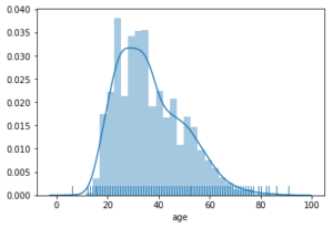
Seaborn allows us plot distribution plots with added features that beat any other visualization library. We can add Kernel Density Estimates Plots (KDE) and a rug of the actual values of the variables. In the example below, we look at the distribution of victims’ age in the police shooting dataset with a kernel density plot and a rug of the variable

'''visualize the dsitribution of victims age in the police shooting dataset with a kernel density plot and a rug of the variables''' 

sns.distplot(police_killings['age'].dropna(), kde=True, rug=True)

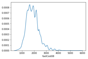
We can also decide to plot only the KDE as shown below:

sns.distplot(vehicles['fuelCost08'].dropna(), hist = False)

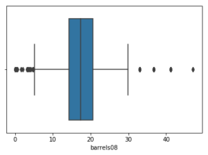
We can also plot boxplots as seen below. The plot is a boxplot of barrels in the vehicles dataset

sns.boxplot(vehicles['barrels08'].dropna())

For Categorical Variables:

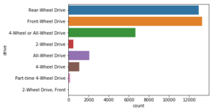
For categorical variables, we can use countplots in Seaborn to visualize the frequency of each category of a variable as shown below:

Here, we view a count of the type of wheel drives:

sns.countplot(y="drive", data=vehicles)

Here, we view a count of the manner of death in the police killings:

sns.countplot(x='manner_of_death', data=police_killings)

I will continue the post explaining more visualization techniques.

I have shared the iPython code here

See you next post ?