OLS and Logistic Regression Models in R

We use linear models primarily to analyse cross-sectional data; i.e. data collected at one specific point in time across several observations. We can also use such models with time series data, but need to be cautious of issues such as serial correlation.

Data can generally take on one of three formats:

• Nominal: A variable that is classified by certain categories that have no particular ordering, e.g. male or female, black or white, etc.
• Ordinal: Variables that are classified according to a ranking system; e.g. rating your favourite food, with a rating of 1 being the lowest and 10 being the highest.
• Interval:
  A variable where the distance between two observations is continuous and not subject to a particular category, e.g. temperature, speed, etc.

Linear Modelling: Ordinary Least Squares regressions

Let us first start with Ordinary Least Squares regressions, which is a common type of linear model used when the dependent variable is either in interval or scale form. To run this type of regression in R, we use the lm

Using an example, we wish to analyze the impact of the explanatory variables capacity, gasoline, and hours on the dependent variable consumption.

Essentially, we wish to determine the gasoline spend per year (in $) for a particular vehicle based on different factors.

Accordingly, our variables are as follows:

• consumption: Spend (in $) on gasoline per year for a particular vehicle
• capacity: Capacity of the vehicle’s fuel tank (in litres)
• price: Average cost of fuel per pump
• hours: Hours driven per year by owner

The purpose of Ordinary Least Squares is to reveal the effect on the dependent variable when the independent variable is changed by 1 unit. For example, when we increase X by 1 unit, by how many units does X increase/decrease?

The Ordinary Least Squares regression has the following structure:

Dependent Variable = Intercept + X1 + X2 + ... + Xn + Error Term

We denote our independent variables by X. The intercept is the minimum value of the dependent variable if all independent variables are set to 0. We interpret our error term as the degree of variation in the dependent variable not explained by our model.

Load data

Firstly, let’s load our data (gasoline.csv) and partition into training and test data:

# Set working directory to where csv file is locatedsetwd("/home/michaeljgrogan/Documents/a_documents/computing/data science/datasets")

# Read the datamydata<- read.csv("gasoline.csv")attach(mydata)

df<-data.frame(consumption,capacity,gasoline,hours)attach(df)

train=head(df,32)test=head(df,8)

Now, we can generate our regression on the training data:

Ordinary Least Squares: Regression and Output

> reg1 <- lm(consumption ~ capacity + price + hours, data=train)> summary(reg1)

Call:lm(formula = consumption ~ capacity + price + hours, data = train)

Residuals:    Min      1Q  Median      3Q     Max -333.40  -67.65    5.96   75.20  144.93 

Coefficients:             Estimate Std. Error t value Pr(>|t|)  (Intercept) 275.18620  663.33899   0.415   0.6814  capacity     -6.54492    4.80236  -1.363   0.1838  price       220.55502   79.89369   2.761   0.0101 *hours         0.04849    0.02387   2.032   0.0518 .---Signif. codes:  0 ‘***’ 0.001 ‘**’ 0.01 ‘*’ 0.05 ‘.’ 0.1 ‘ ’ 1

Residual standard error: 108.9 on 28 degrees of freedomMultiple R-squared:  0.5419,Adjusted R-squared:  0.4928 F-statistic: 11.04 on 3 and 28 DF,  p-value: 5.883e-05

When we yield our output, we see the gasoline and hours variables are deemed statistically significant. This means that these variables are indicated to have a material effect on consumption.

Model Interpretation

Y = 275.18 - 6.544(capacity) + 220.55(price) + 0.048(hours)

According to the output:

• A 1 unit increase in the capacity of the fuel tank leads to a drop of 6.544 units of gasoline consumption.
• An increase of 1 unit in gasoline prices is correlated a 220.55 unit increase in consumption. This could indicate that vehicles that require a more expensive fuel type fuel type typically see a higher spend on fuel by the driver.
• When we increase the hours driven by 1 unit, the consumption increases by 0.048. Cars that are driven for longer periods may be more fuel-efficient, and this is why the increase in consumption may not be as high as expected.

Additionally, we have an R-Squared value of 0.5419 — meaning that 54.19% of the variation in stock returns is allegedly “explained” by this model.

We now test for multicollinearity and heteroscedasticity to ensure that the statistical readings of our model are reliable. If we find high t-statistics and R-Squared values in our output, it means our standard errors may be biased.

Multicollinearity

• Multicollinearity exists when two independent variables in the linear model are significantly related, to the extent that inclusion of both variables in a regression model may skew our OLS estimates.
• To test for multicollinearity, we use the Variance Inflation Factor (VIF) test across our independent variables. We determine that a reading of 5 or greater indicates the presence of multicollinearity.
• From the below, given that we did not calculate VIF readings of 5 or greater, this indicates that our model does not suffer from multicollinearity.

> library(car)> vif(reg1)capacity price hours 2.003143 1.054277 1.974485

Heteroscedasticity

• Heteroscedasticity occurs when we have an uneven variance across our observations.
• For instance, let us assume that we have a mixture of small and large-cap stocks across our observations. This means that we have an uneven variance; i.e. returns will move unevenly depending on the size of the company.
• We test for heteroscedasticity using the Breusch-Pagan test at the 5% level of significance. With a p-value of 0.278 our test is insignificant and this indicates that heteroscedasticity is not present in our model.

> library(lmtest)> bptest(reg1)

studentized Breusch-Pagan test

data:  reg1BP = 3.8512, df = 3, p-value = 0.278

Now that we have generated our regression output, we would now like to:

1. Generate predictions using the independent variables in the test data
2. Compare these to the actual data and calculate the mean squared error

> test_predict<-as.numeric(predict(reg1,test))> test_predict[1] 1376.399 1407.636 1444.875 1423.572 1445.335 1487.809 1386.498 1565.968> mse=(test_predict-test$consumption)/test$consumption> mse[1]  0.31965342  0.07699799  0.08800835  0.06157486  0.03164490  0.05818546 -0.03177502[8]  0.09278988

From the above, we see that the most of our observations have a deviation of below 10%, indicating that our model has a significant degree of ability to predict the dependent variable.

In the real world, we would want to have significantly more than 40 observations to test our hypotheses more rigorously. However, the above is primarily to illustrate the theoretical aspects of a linear regression, and how we would run one in R.

Generalized Linear Modelling: Binomial Logistic Regressions

A binomial logistic regression is a type of Generalized Linear Model, run using the glmcommand in R. The purpose of a binomial logistic regression is to regress a dependent variable that can only take on finite values. In this instance, we wish to calculate an odds ratio for our regression — i.e. what is the probability that a stock will increase its dividend payments based on another event taking place? Here, we use the glm function to construct a binomial logistic regression in R.

This generalized linear regression model is used when we wish to analyse a regression where our dependent variable is a nominal variable. For instance, in the previous example using Ordinary Least Squares we saw that stock returns was an interval variable as it could take on a continuous range. However, let us assume that we now wish to have a nominal (or dummy) variable as our dependent variable. We will use the dividendinfo.csv dataset. Here is the structure of our variables within the glm model:

Dependent Variable (Y)

• dividend: If the company pays dividends currently it is given a ranking of 1. If the company does not pay dividends, it is given a ranking of 0.

Independent Variables (X)

• fcfps: Free cash flow per share (in $)
• earnings_growth: Earnings growth in the past year (in %)
• de: Debt to Equity ratio
• mcap: Market Capitalization of the stock
• current_ratio: Current Ratio (or Current Assets/Current Liabilities)

Using the binomial logistic regression, we wish to analyse the likelihood of a company paying a dividend based on changes in the above independent variables. Note that in this case, we are not looking to obtain a specific coefficient value but rather an odds ratio; a ratio that tells us the likelihood of a dividend payment based on any independent variable.

glm Regression Model

> summary(logreg)

Call:glm(formula = dividend ~ fcfps + earnings_growth + de + mcap +     current_ratio, family = "binomial", data = train)

Deviance Residuals:      Min        1Q    Median        3Q       Max  -2.11568  -0.00171   0.00000   0.00257   1.89044  

Coefficients:                 Estimate Std. Error z value Pr(>|z|)   (Intercept)     -31.84319   10.15009  -3.137  0.00171 **fcfps             2.34051    0.86664   2.701  0.00692 **earnings_growth   0.12416    0.04347   2.856  0.00429 **de               -2.02328    0.86428  -2.341  0.01923 * mcap              0.03698    0.01186   3.118  0.00182 **current_ratio     9.12311    3.15168   2.895  0.00380 **---Signif. codes:  0 ‘***’ 0.001 ‘**’ 0.01 ‘*’ 0.05 ‘.’ 0.1 ‘ ’ 1

(Dispersion parameter for binomial family taken to be 1)

    Null deviance: 221.782  on 159  degrees of freedomResidual deviance:  27.363  on 154  degrees of freedomAIC: 39.363

Number of Fisher Scoring iterations: 10

Note that we do not have an R-Squared statistic in this instance — given far less variance in our dependent variable an R-Squared statistic would prove unreliable.

To calculate an odds ratio, it is necessary to get the exponent of the independent variable in question — since a binomial logit model will show an exponential rather than a linear trend line. Since our fcfps variable is statistically significant at the 5% level — this is the variable that we will exponentiate:

> exp(2.34051)[1] 10.38656

We have calculated a log odds ratio of 10.386:1, which means that the odds of a dividend increase are 10.386 times greater than the odds of the dividend staying at the same rate or decreasing.

Moreover, as the following source elaborates in more detail, we can convert these odds into a probability as follows:

exp / (1+exp) = probability

In the case of a log odds ratio of 10.386, we yield a probability of 91.21% chance of a dividend increase, where 10.38656/(1+10.38656) = 0.9121.

ROC Curve

As from the above, a logistic regression was generated on the training data. However, we wish to analyse whether the regression that we generated is accurate in classifying whether a stock pays a dividend or not.

pred1 <- predict(logreg1, test, type="response")y_pred1_num <- ifelse(pred1 > 0.5, 1, 0)y_pred1 <- factor(y_pred1_num, levels=c(0, 1))plot(roc(test$dividend,y_pred1_num))rocPred <- roc(test$dividend,y_pred1_num)auc1 <- auc(rocPred)print(auc1)

An ROC curve allows us to determine whether the logistic regression is more accurate at predicting the correct 0 or 1 value as opposed to simply taking a random guess. Specifically, we will interpret the AUC (area under the curve) as a measure of such accuracy.

Here is a plot of the ROC curve:

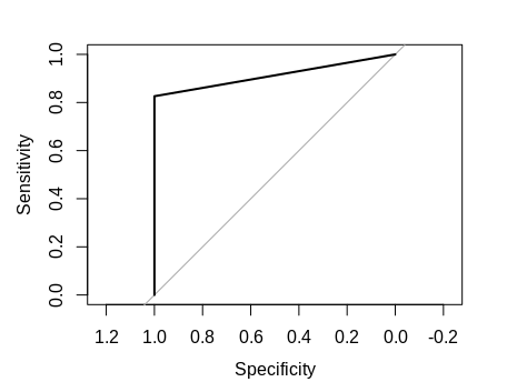
We also generate an AUC of 91.3%:

> print(auc1)Area under the curve: 0.913

Essentially, an AUC of 91.3% means that the logistic regression is quite accurate at predicting the correct 1 or 0 value as opposed to a random guess. For instance, if we had an AUC of 0.5 (or 50%), then it would mean that our logistic regression model is no more accurate than a random guess in predicting the value of the binary dependent variable.

Conclusion

In this tutorial, you have learned:

• How to generate linear and logistic regressions in R
• Corrections for OLS violations
• How to gauge accuracy of logistic regressions with ROC curves

Many thanks for reading, and if you’re interested in how we can generate linear and logistic regression models in Python, you can read that article here.