Datacamp Learning

Logistic regression in R

Building simple logistic regression models

The donors dataset contains 93,462 examples of people mailed in a fundraising solicitation for paralyzed military veterans. The donated column is 1 if the person made a donation in response to the mailing and 0 otherwise. This binary outcome will be the dependent variable for the logistic regression model.
The remaining columns are features of the prospective donors that may influence their donation behavior. These are the model’s independent variables.
When building a regression model, it is often helpful to form a hypothesis about which independent variables will be predictive of the dependent variable. The bad_address column, which is set to 1 for an invalid mailing address and 0 otherwise, seems like it might reduce the chances of a donation. Similarly, one might suspect that religious interest (interest_religion) and interest in veterans affairs (interest_veterans) would be associated with greater charitable giving.
In this exercise, you will use these three factors to create a simple model of donation behavior.

# Examine the dataset to identify potential independent variables
str(donors)
# Explore the dependent variable
table(donors$donated)
# Build the donation model
donation_model <- glm(donated~bad_address+interest_religion+interest_veterans,data = donors, family = "binomial")
# Summarize the model results
 

summary(donation_model)

Making a binary prediction

In the previous exercise, you used the glm() function to build a logistic regression model of donor behavior. As with many of R’s machine learning methods, you can apply the predict() function to the model object to forecast future behavior. By default, predict() outputs predictions in terms of log odds unless type = “response” is specified. This converts the log odds to probabilities.

Because a logistic regression model estimates the probability of the outcome, it is up to you to determine the threshold at which the probability implies action. One must balance the extremes of being too cautious versus being too aggressive. For example, if you were to solicit only the people with a 99% or greater donation probability, you may miss out on many people with lower estimated probabilities that still choose to donate. This balance is particularly important to consider for severely imbalanced outcomes, such as in this dataset where donations are relatively rare.

# Estimate the donation probability
donors$donation_prob <- predict(donation_model, type = "response")

# Find the donation probability of the average prospect
mean(donors$donated)

# Predict a donation if probability of donation is greater than average (0.0504)
donors$donation_pred <- ifelse(donors$donation_prob > 0.0504, 1, 0)

# Calculate the model's accuracy
mean(donors$donation_pred == donors$donated)

Calculating ROC Curves and AUC

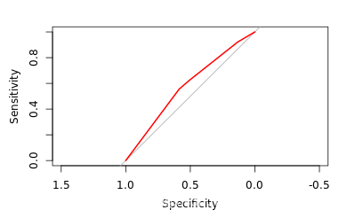
The previous exercises have demonstrated that accuracy is a very misleading measure of model performance on imbalanced datasets. Graphing the model’s performance better illustrates the tradeoff between a model that is overly agressive and one that is overly passive.

In this exercise you will create a ROC curve and compute the area under the curve (AUC) to evaluate the logistic regression model of donations you built earlier.

# Load the pROC package
library(pROC)

# Create a ROC curve
ROC <- roc(donors$donated,donors$donation_prob)

# Plot the ROC curve
plot(ROC, col = 'blue')

# Calculate the area under the curve (AUC)
auc(ROC)

Coding categorical features

Sometimes a dataset contains numeric values that represent a categorical feature.
In the donors dataset, wealth_rating uses numbers to indicate the donor’s wealth level:
0 = Unknown
1 = Low
2 = Medium
3 = High
This exercise illustrates how to prepare this type of categorical feature and the examines its impact on a logistic regression model.
Factors have specific sequence. ‘Relevel’ means move up the pointed factor to the first postion.

# Convert the wealth rating to a factor
donors$wealth_rating <- factor(donors$wealth_rating, levels = c(0,1,2,3), labels = c('Unknown','Low','Medium','High'))
donors$wealth_rating

# Use relevel() to change reference category
donors$wealth_rating <- relevel(donors$wealth_rating, ref = 'Medium')

# See how our factor coding impacts the model
summary(glm(donated~wealth_rating,data=donors,family='binomial'))

Handling missing data

Some of the prospective donors have missing age data. Unfortunately, R will exclude any cases with NA values when building a regression model.
One workaround is to replace, or impute, the missing values with an estimated value. After doing so, you may also create a missing data indicator to model the possibility that cases with missing data are different in some way from those without.

# Find the average age among non-missing values
summary(donors$age)

# Impute missing age values with mean(age)
donors$imputed_age <- ifelse(is.na(donors$age), 61.65, donors$age)

# Create missing value indicator for age
donors$missing_age <- ifelse(is.na(donors$age), 1, 0)

#Building a more sophisticated model
One of the best predictors of future giving is a history of recent, frequent, and large gifts. In marketing terms, this is known as R/F/M:
Recency
Frequency
Money
Donors that haven’t given both recently and frequently may be especially likely to give again; in other words, the combined impact of recency and frequency may be greater than the sum of the separate effects.
Because these predictors together have a greater impact on the dependent variable, their joint effect must be modeled as an interaction.

# Build a recency, frequency, and money (RFM) model
rfm_model <- glm(donated ~ recency * frequency + money, data = donors, family = "binomial")

# Summarize the RFM model to see how the parameters were coded
summary(rfm_model)

# Compute predicted probabilities for the RFM model
rfm_prob <- predict(rfm_model, data = donors, type = "response")

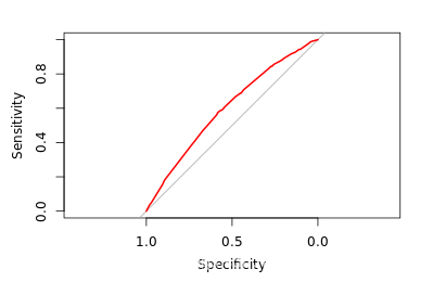
# Plot the ROC curve for the new model
library(pROC)
ROC <- roc(donors$donated, rfm_prob)
plot(ROC, col = "red")
auc(ROC)

Building a stepwise regression model

In the absence of subject-matter expertise, stepwise regression can assist with the search for the most important predictors of the outcome of interest.
In this exercise, you will use a forward stepwise approach to add predictors to the model one-by-one until no additional benefit is seen.

# Specify a null model with no predictors
null_model <- glm(donated ~ 1, data = donors, family = "binomial")

# Specify the full model using all of the potential predictors
full_model <- glm(donated ~ ., data = donors, family = "binomial")

# Use a forward stepwise algorithm to build a parsimonious model
step_model <- step(null_model, scope = list(lower = null_model, upper = full_model), direction = "forward")

Merci, c’est tout.