2D Convolutions

Convolutions gained significant popularity after successes in the field of Computer Vision, on tasks such as image classification, object detection and instance segmentation. Since these tasks use images as inputs, and natural images usually have patterns along two spatial dimensions (of height and width), it’s more common to see examples of 2D Convolutions than 1D and 3D Convolutions. We’ll look at those cases in the next post, but let’s just stick to 2D Convolutions for now.

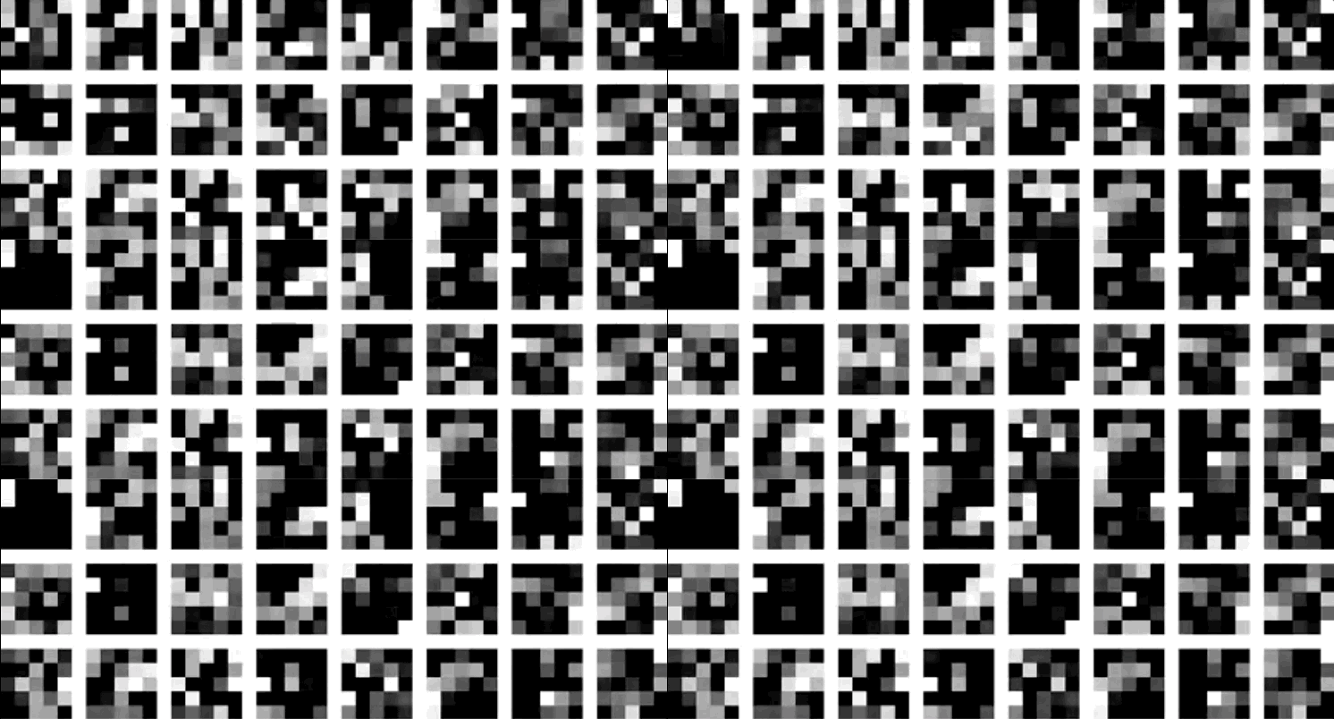
One of the most important components of a convolution operation is the kernel (a.k.a filter). You define the size of the kernel, and for 2D Convolutions (applied to single dimensional input array), the kernel will be a 2D array too: 3x3 is a common choice. Although the convolution is just a mathematical operation at heart, an interpretation of the kernel is that it’s the ‘spatial feature’ you’re looking to detect in the input. Some of the most simple spatial features represent edges of objects. And as you apply convolutions over and over again (layer after layer), you can create more abstracted spatial features: edges can be combined to define curves, then curves into an eye, and two eyes and a snout to define dog faces! A good way to visualise the spatial features captured by a kernel is to plot the image patches from a dataset that maximise the outputs of convolution with that kernel: see Figure 1 below.

Watch out! We’re visualising image patches here (i.e. regions of images), and not the kernel values. Although first layer kernels could be interpreted directly, things get progressively more abstract with kernels from later convolutional layers.

So how do you choose the best kernel?

Once upon a time, you’d handcraft your own kernels; often basing them on pre-existing work and examples (see here for some simple cases). As you can imagine, this process could take a huge amount of time and is really tricky for kernels of convolutions that are deep in the network. And previously, there wasn’t a clear path or strategy to find the optimal values.

Stochastic gradient descent to the rescue! Our lives are much easier since the advent of neural networks and the back-propagation algorithm. Using the gradient of the loss with respect to each parameter (a.k.a weight) in the kernel, we can iteratively improve our kernels a batch of data at a time. So in the deep-learning paradigm, we just initialise the kernel with random values and optimise. And this is why people often say that deep-learning models learn the optimal features to extract as part of the learning process.

And how are the kernels used?

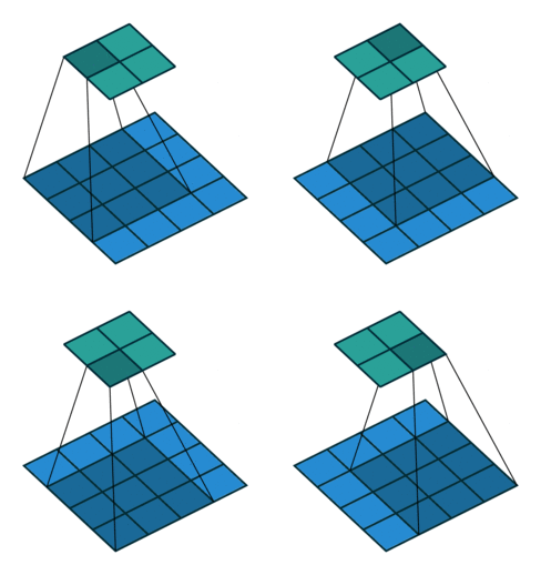
Some of the best visualisations of 2D convolutions I have seen are from Vincent Dumoulin & Francesco Visin. In their diagram below, we see a kernel (dark blue region) slide across the input matrix (blue) and produce and output matrix (green). With 2D Convolutions we slide the kernel in two directions: left/right and up/down. Although the movement of the kernel is shown clearly, the operation that happens at each step isn’t explained, and it would be useful to see some tangible examples using real numbers.

About time we saw some numbers!

We’ll implement this in Excel to see how it’s done and then take a look at the MXNet Gluon code that can replicate this scenario. So let’s generate some dummy data for our input matrix and our convolution’s kernel and apply the convolution operation to calculate our output.

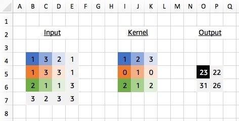
We start by applying our 3x3 kernel to the equivalently sized 3x3 region in the top left corner of our input matrix. We calculate what’s called the ‘dot product’ of the input region and the kernel, which is just the element-wise product (i.e. multiply the colour pairs) followed by a global sum to obtain a single value. So in this case:

(1*1)+(3*2)+(2*3)+(1*0)+(3*1)+(3*0)+(2*2)+(1*1)+(1*2) = 23

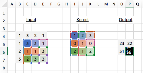
And similarly for other regions of the input (take the 3x3 region in the bottom right corner of our input matrix for example) we use the same kernel values each time for our dot product calculation. And this time we show the Excel formula used to calculate the output of 26.

About time we saw some code!

With MXNet Gluon it’s really simple to create a convolutional layer (technically a Gluon Block) to perform the same operation as above.

import mxnet as mx

conv = mx.gluon.nn.Conv2D(channels=1,                          kernel_size=(3,3))

We use Conv2D because we want to slide the kernel in two spatial dimensions: left/right and up/down. Check out the next blog post for more information on Conv1D and Conv3D, where we slide the kernel in fewer or more dimensions. Specifying channels=1 since we are only applying a single kernel in this case, we can now pass our input into the conv block using a predefined kernel.

input_data = mx.nd.array(((1,3,2,1),                          (1,3,3,1),                          (2,1,1,3),                          (3,2,3,3)))

kernel = mx.nd.array(((1,2,3),                      (0,1,0),                      (2,1,2)))

# see appendix for definition of `apply_conv`output_data = apply_conv(input_data, kernel, conv)print(output_data)

# [[[[23. 22.]#    [31. 26.]]]]# <NDArray 1x1x2x2 @cpu(0)>

Our apply_conv function is used to set the kernel weights of the convolutional layer to predefined values, and apply the operation. As mentioned previously, we don’t often do this in practice since the whole purpose of training our network is to determine the best kernel weights to use. But for understanding how the convolution works it’s really useful to be able to set the kernel weights. Check out the Appendix for the implementation.

2D Convolutions with Padding

You may have noticed in the last example that our output matrix dimensions (2x2) were different from the input matrix dimensions (4x4), since it was only possible to slide the kernel by one element in each direction. We would expect to lose 2 elements from the output in each dimension using a 3x3 kernel. Using a technique called padding we can maintain the spatial dimensions through the convolution operation.

Although different padding techniques exist, one of the most common methods is to pad the input with 0s by a defined number of elements in every direction (both before and after). With a 3x3 kernel we need to pad by one element in every direction to maintain the dimensions, and we see the output is now 4x4.

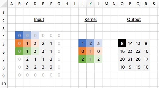
Once again, this case is simple to replicate in MXNet Gluon. We just specify the padding as a tuple for the amount of padding we want to add in each of the spatial directions (both before and after).

conv = mx.gluon.nn.Conv2D(channels=1,                          kernel_size=(3,3),                          padding=(1,1))

output_data = apply_conv(input_data, kernel, conv)print(output_data)

# [[[[ 8. 14. 13.  8.]#    [16. 23. 22. 10.]#    [20. 31. 26. 17.]#    [10.  9. 15. 10.]]]]# <NDArray 1x1x4x4 @cpu(0)>

2D Convolutions with Stride

So far we’ve seen examples of the kernel sliding across the input matrix one element at a time in each direction, but we can actually change the behaviour of this movement. Stride defines how much of a jump we want to make between evaluations, and is an effective method for reducing the spatial dimensions while avoiding overlap between the evaluations. With a stride of 2 (also denoted 2x2), notice how the kernel jumps 2 elements at a time in each direction in the diagram below.

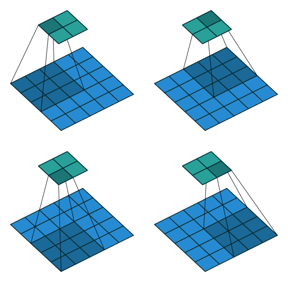
We extend our input data in Excel to 5x5 to match the diagram but use the same kernel and apply it in the same way as before. Our change is to only evaluate the dot product at every other position hence giving us an expanded output (containing gaps) that we need to reduce to obtain the final output.

Similarly, in MXNet Gluon we create a new input_data array:

input_data = mx.nd.array(((1,3,2,1,2),                          (1,3,3,1,2),                          (2,1,1,3,1),                          (3,2,3,3,2),                          (2,3,1,2,2)))

And create a Conv2D layer, with strides set to a tuple containing the number of elements to step in each of the spatial dimensions, in this case (2,2).

conv = mx.gluon.nn.Conv2D(channels=1,                          kernel_size=(3,3),                          strides=(2,2))

output_data = apply_conv(input_data, kernel, conv)print(output_data)

# [[[[23. 18.]#    [18. 21.]]]]# <NDArray 1x1x2x2 @cpu(0)>

Note: it is possible to combine stride with padding. Adding padding=(1,1) to the example above would give us a 3x3 output. Give it a try and experiment with other combinations!

2D Convolutions with Dilation

Using our 3x3 kernel, we can find local patterns since we are using values from a tight neighbourhood of 9 points. But we have a limited ‘receptive field’ and we might miss patterns that are happening at a larger scale. One solution for this problem is to stack convolutional layers (with stride or max pooling), but another potentially more efficient way to capture these effects is through dilation of our kernel. Sometimes called an atrous convolution.

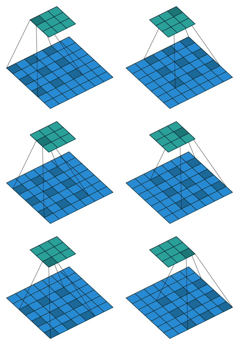
Our kernel appears expanded in the diagram above because we are using separated elements of our input matrix in the calculation of the dot product. Using a dilation factor of 2 (also denoted 2x2) we take a step of 2 between elements in our input matrix, thus leaving a gap of 1 between each. We see the same effect in Excel too: once again using colour pairs for the element-wise products.

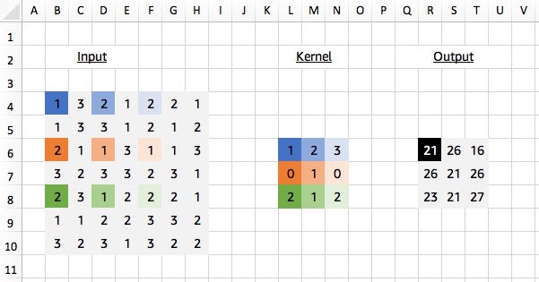
We can replicate this in MXNet Gluon, by first creating the same 7x7 array:

input_data = mx.nd.array(((1,3,2,1,2,2,1),                          (1,3,3,1,2,1,2),                          (2,1,1,3,1,1,3),                          (3,2,3,3,2,3,1),                          (2,3,1,2,2,2,1),                          (1,1,2,2,3,3,2),                          (3,2,3,1,3,2,2)))

And then creating a Conv2D layer, with dilation set to a tuple containing the number of elements to step in each of the spatial dimensions, in this case (2,2).

conv = mx.gluon.nn.Conv2D(channels=1,                          kernel_size=(3,3),                          dilation=(2,2))

output_data = apply_conv(input_data, kernel, conv)print(output_data)

# [[[[21. 26. 16.]#    [26. 21. 26.]#    [23. 21. 27.]]]]# <NDArray 1x1x3x3 @cpu(0)>

All together now

And lastly, just for fun, let’s combine everything we’ve just learnt into a single example: a 2D convolution with padding, stride and dilation. You might not see these convolution settings in the wild but it helps us double check our understanding of the concepts. We apply a 2D convolution with padding of 2x2, stride of 2x2 and dilation of 2x2, while keeping the same 7x7 input matrix and kernel as before. With Excel:

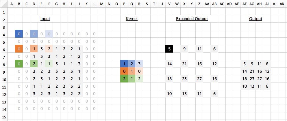
And with MXNet Gluon:

conv = mx.gluon.nn.Conv2D(channels=1,                          kernel_size=(3,3),                          padding=(2,2),                          strides=(2,2),                          dilation=(2,2))

output_data = apply_conv(input_data, kernel, conv)print(output_data)

# [[[[ 5.  9. 11.  6.]#    [14. 21. 16. 12.]#    [18. 23. 27. 16.]#    [10. 13. 11.  6.]]]]# <NDArray 1x1x4x4 @cpu(0)>

Get experimental

All the examples shown in this blog posts can be found in this MS Excel Spreadsheet (or Google Spreadsheet). Click on the cells of the output to inspect the formulas and try different kernel values to change the outputs. After replicating your results in MXNet Gluon, I think you can officially add ‘convolutions’ as a skill on your LinkedIn profile!

Up next

We’ll be taking a look at some of the more advanced usages of convolutions in the next few blog posts. We’ll start by extending what we already know to 1D and 3D Convolutions. And then work up to multi-channel and transposed convolutions.

Appendix: