Multi-Channel Convolutions explained with… MS Excel!

We’ve looked at 1D Convolutions, 2D Convolutions and 3D Convolutions in previous posts of the series, so in this next post we’re going to be looking at 4D Convolutions, 5D Convolutions and 6D Convolutions…

Just kidding! We’re going to be taking a look a something much more useful, and much easier to visualise with MS Excel. We start with convolutions applied to multiple input channels and then we look at convolutions that return multiple output channels. Simple, in MXNet Gluon!

Multiple Input Channels

So far in this convolution series we’ve been applying:

• 1D Convolutions to 1 dimensional data (temporal)
• 2D Convolutions to 2 dimensional data (height and width)
• 3D Convolutions to 3 dimensional data (height, width and depth)

You’ll see an obvious pattern here, but this simple correspondence hides an important detail. Our input data usually defines multiple variables at each position

Conv1D with Multiple Input Channels

As a sugar-coated example, let’s take the case of ice cream sales forecasting. Our input might be defined at daily intervals along our temporal dimension and have normalised values for the product’s price, marketing spend, outside temperature and whether it was the weekend or not. 4 channels

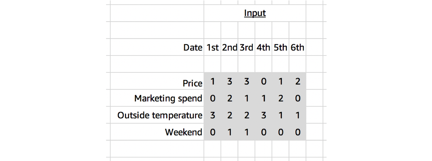
Although the input data looks like it’s two dimensional, only one of the dimensions is spatial. We’d only expect to find patterns in a local neighbourhood of values through time, and not across a local neighbourhood the channel variables. Starting with a random order of 4 variables (A, B, C, D), we would not expect to find a similar spatial relationship between A&B, B&C and C&D (if we set a kernel shape of 2 along this dimension).

So for this reason, when working with multi-channel temporal data, it’s best to use a 1D Convolution; even though the data looks two dimensional.

Applying a 1D Convolution (with kernel size of 3), our kernel will look different to the single channel case shown in the last post. Given we have 4 input channels this time, our kernel will be initialised with 4 channels too. So even though we are using a 1D Convolution, we have a 2D kernel! A 1D Convolution just means we slide the kernel along one dimension, it doesn’t necessarily define the shape of the kernel, since that depends on the shape of the input channels too.

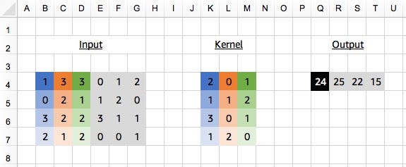
Advanced: a 2D Convolution with kernel shape (3,4) would be equivalent in this situation, but with a 1D Convolution you don’t need to specify the channel dimension. We usually rely on shape inference for this (i.e. after passing the first batch of data), but we can manually specify the number of input channels with in_channels. When adding padding, stride and dilation to the equation, the equivalence between 2D and 1D Convolutions might not hold.

# define input_data and kernel as above# input_data.shape is (4, 6)# kernel.shape is (4, 3)

conv = mx.gluon.nn.Conv1D(channels=1, kernel_size=3)

# see appendix for definition of `apply_conv`output_data = apply_conv(input_data, kernel, conv)print(output_data)

# [[[24. 25. 22. 15.]]]# <NDArray 1x1x4 @cpu(0)>

Our code remains unchanged from the single input channel case.

Just before we wrap up with 1D Convolutions, it’s worth mentioning another common use-case. One of the first stages in many Natural Language Processing models is to convert a sequence of raw text into a sequence of embeddings, either character, word or sentence embeddings. At every time step we now have an embedding with a certain number of values (e.g. 128) that each represent different attributes about the character, word or sentence. We should think about these just as with the time series example, and treat them as channels. Since we’ve just got channels over time, a 1D Convolution is perfect for picking up on useful local temporal patterns.

Conv2D with Multiple Input Channels

Colour images are a great example of multi-channel spatial data too. We usually have 3 channels to represent the colour at each position: for the intensities of red, green and blue colour. What’s new this time though, is that we’re dealing with two spatial dimensions: height and width.

Our kernel will adjust to the channels accordingly and even though we define a 3x3 kernel, the true dimensions of the kernel when initialised will be 3x3x3, since we have 3 input channels. Since we’re back to 3 dimensions again, let’s take a look at a three.js diagram first before blowing our minds with MS Excel.

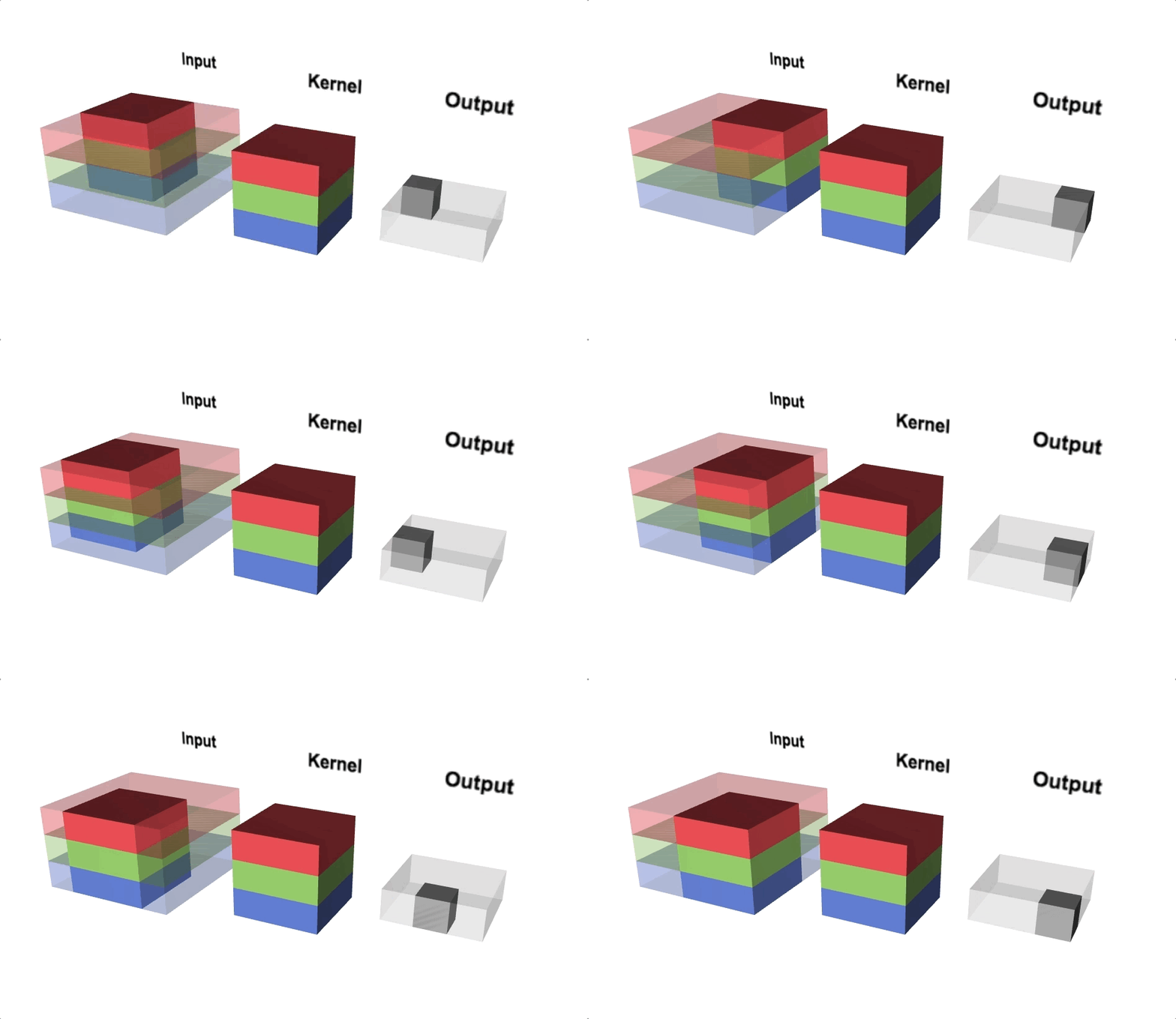
With the diagram above you should think about viewing from above if you wanted to view the actual image, but we’re interested in seeing the channels, hence why we’re looking from a slide angle. Check out this link for an interactive version of the diagram above. One interesting observation is that each ‘layer’ of the kernel interacts with a corresponding channel of the input.

We can actually see this in more detail when looking at MS Excel.

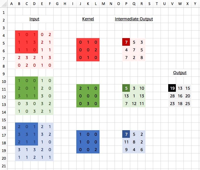
Viewed like this, we think as if each channel has its own 3x3 kernel. We apply each “layer” of the kernel to the corresponding input channel and obtain intermediate values, a single value for each channel. Our final step is sum up these values, to obtain our final result for the output. So ignoring 0s we get:

red_out = (3*2)+(1*1) = 7

green_out = (1*2)+(1*3) = 5

blue_out = (2*1)+(3*1)+(1*2) = 7

output = red_out + green_out + blue_out = 7+5+7 = 19

We don’t actually calculate these intermediate results in practice but it shows the initial separation between channels. A kernel still looks at patterns across channels though, since we have the cross channel summation at the end.

Advanced: a 3D Convolution with kernel shape (3,3,3) would be equivalent in this situation, but with a 2D Convolution you don’t need to specify the channel dimension. Again, we usually rely on shape inference for this (i.e. after passing the first batch of data), but we can manually specify the number of input channels with in_channels. When adding padding, stride and dilation to the equation, the equivalence between 3D and 2D Convolutions might not hold.

# define input_data and kernel as above# input_data.shape is (3, 5, 5)# kernel.shape is (3, 3, 3)

conv = mx.gluon.nn.Conv2D(channels=1, kernel_size=(3,3))

output_data = apply_conv(input_data, kernel, conv)print(output_data)

# [[[[19. 13. 15.]#    [28. 16. 20.]#    [23. 18. 25.]]]]# <NDArray 1x1x3x3 @cpu(0)>

Code in MXNet Gluon looks the same as with a single channel input, but notice that the shape of the kernel is (3,3,3) because we have a kernel applied to an input with 3 channels and it has a height of 3 and a width of 3. Our layout for the kernel is therefore (in_channels, height, width).

Multiple Output Convolutions

All the way back in the first blog post of the series we introduced the convolution as a feature detector, with the kernel defining the type of feature we wanted to detect. So far, in all of our examples, we’ve been using a single kernel as part of our convolution, meaning that we’ve just been looking for a single feature. Clearly for tasks as complex as image classification, object detection and segmentation we need to be looking at more than one feature at each layer of the network.

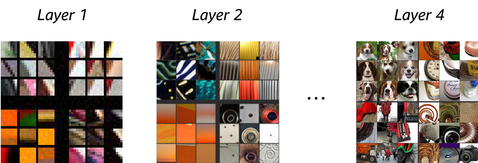
Starting with the first convolutional layers, it might be useful to detect edges at different angles and different colour contrasts (an example of multiple input channel kernels that we’ve just learnt about). And then in later layers, it might be useful to detect spirals, as well as dog faces (always useful!).

Computationally, it’s very easy to add multiple output channels. We just repeat the whole process from before for as many output channels as we require, each time with a different and independent kernel, and just stack all of the outputs. Voilà!

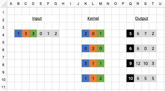
Compare this with the Figure 2 from the last blog post. Our first kernel is the same as in that example and we get the same output (of shape 1x4), but this time we add 3 more kernels and get an final output of shape 4x4.

As usual, this is simple to add to our convolutions in MXNet Gluon. All we need to change is the channels parameter and set this to 4 instead of 1.

conv = mx.gluon.nn.Conv1D(channels=4, kernel_size=3)

Advanced: We previously mentioned the similarly named parameter called in_channels. It’s important to note the difference. in_channels is used if you want to specify the number of channels expected in the input data, instead of using shape inference (by passing the first batch of data). channels is used to specify the number of output channels required, i.e. the number of kernels/filters.

# define input_data and kernel as above# input_data.shape is (1, 6)# kernel.shape is (4, 1, 3)

output_data = apply_conv(input_data, kernel, conv)print(output_data)

# [[[ 5.  6.  7.  2.]#   [ 6.  6.  0.  2.]#   [ 9. 12. 10.  3.]#   [10.  6.  5.  5.]]]# <NDArray 1x4x4 @cpu(0)>

Once upon a time, back in the last post, our 1D Convolution’s kernel was also 1D. When we had multiple input channels, we had to add an extra dimension to the handle this. And now we’re looking at multiple output channels, we’ve got to add another! Which takes us up to 3D in total for a 1D Convolution. We’ve had these dimensions all along (apologies for hiding the truth from you again!), but it was simpler to ignore them since they were of unit length and just let apply_conv add them for us.

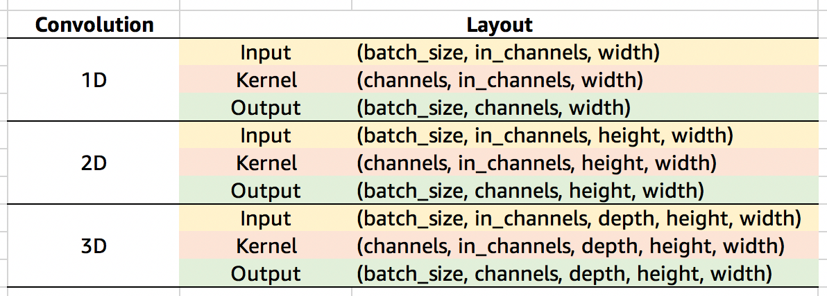
So for the case above we can see our kernel is of shape (4,1,3). We have 4 kernels, each of which is applied to the same input data with 1 channel, and they all have a width of 3 in the temporal dimension. Our layout for the kernel is therefore (channels, in_channels, width). Check the following table for a more complete list of default dimension layouts.

Advanced: Depth-wise Separable Convolutions

The vast majority of convolutions you’ll see in common neural networks architectures will be applied to multiple input channels and return multiple output channels. Computation scales linearly with the number of output channels, but the amount of computation required can still get very large for large in_channels and large channels. As a more efficient alternative, we can use a depth-wise separable convolution. When we looked at multiple input channels (see Figure 5), we showed an intermediate step before the sum across input channels. With depth-wise separable convolutions, you apply a 1x1 convolution instead of the sum. We’ve essentially split the convolution into 2 stages: the first looking at spatial patterns across each channel input individually, and the second looking across channels (but not spatially).

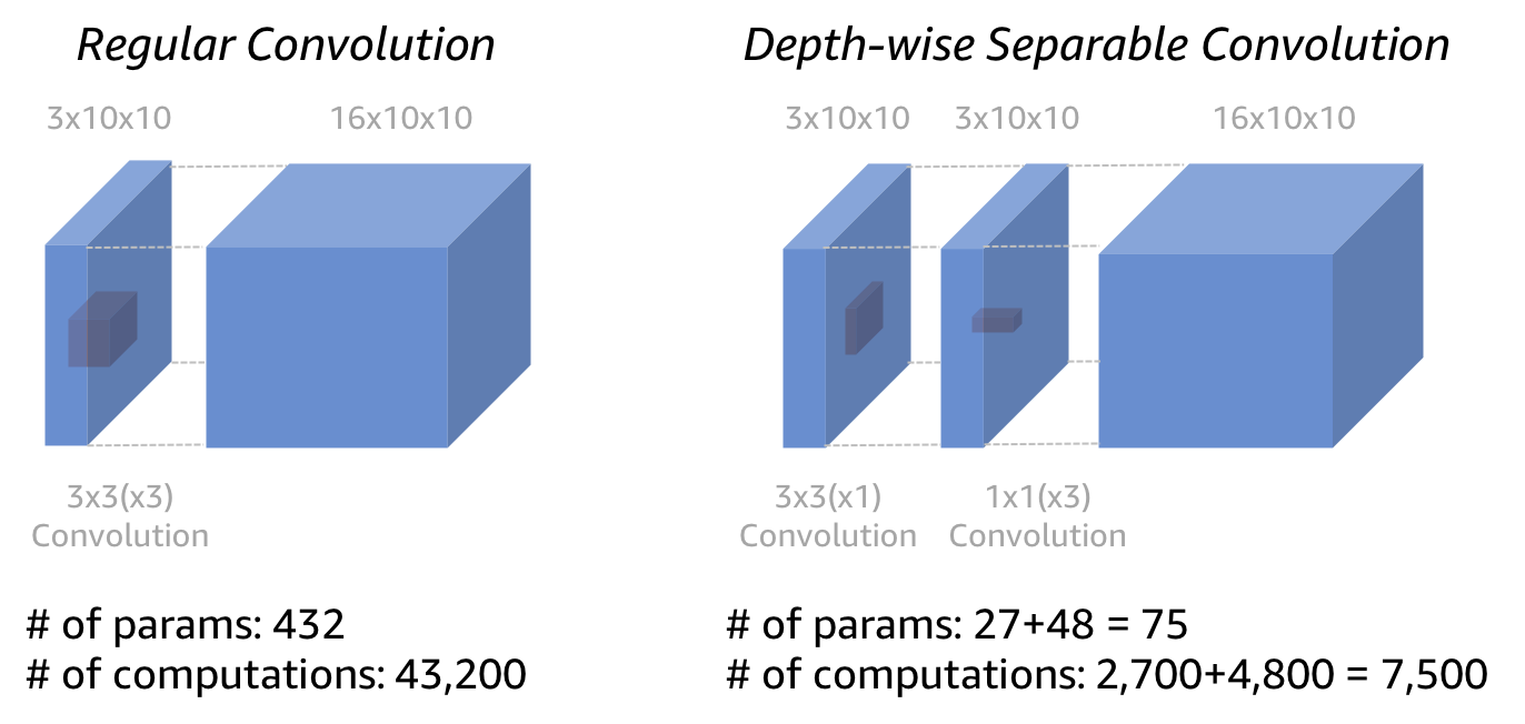
With MXNet Gluon we can use the groups argument of the convolution to specify how we want to partition the operation. Check the MobileNet implementation for MXNet Gluon for an example usage. groups are set to the number of input channels which gives the depth-wise separable convolution.

Get experimental

All the examples shown in this blog posts can be found in these MS Excel Spreadsheets for Conv1D and Conv2D (or on Google Sheets here and here respectively). Click on the cells of the output to inspect the formulas and try different kernel values to change the outputs. After replicating your results in MXNet Gluon, I think you can officially add ‘convolutions guru’ as a title on your LinkedIn profile!

Up next

All good things must come to an end, but not before we’ve understood the Transposed Convolution! In the final blog post of the series we’ll be taking a look at two different mental models for thinking about Transposed Convolutions, and see some practical examples too.

Appendix: