Market dynamics plays a key role in matching guests with hosts in two-sided marketplaces such as Airbnb. Supply and demand vary drastically across different locations, different check in dates and different lead times until check-in. It is important for us to understand and forecast these spatial and temporal trends in order to find better matches for our community of hosts and guests.

In this post, we describe a framework used to model lead time dynamics in order to help hosts price their homes more competitively and improve their earnings potential. We embrace both machine learning (ML) and structural modeling to achieve improved predictive performance and model interpretability.

A Primer on Lead Time Dynamics

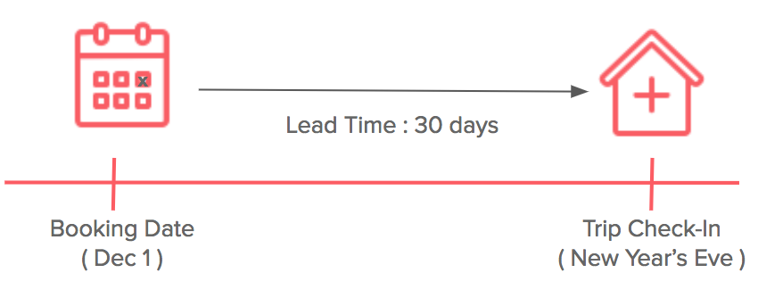
The lead time for a booking refers to the time between the date of booking and the trip check-in date. Taking a trip with a check-in date of New Year’s Eve (December 31) as an example, when a guest books 30 days in advance (on December 1), the booking lead time is 30 days. On the other hand, the booking lead time would be 0 for guests who make a last minute reservation on the day of check-in.

Guests will continue to make bookings for the New Year’s Eve as time progresses and the booking date gets closer and closer to the end of the year. This booking process reflects the inflow of demand and can be treated as a stochastic arrival process. The corresponding distribution of bookings over lead time is the booking lead time distribution.

Why Model the Lead Time Distribution?

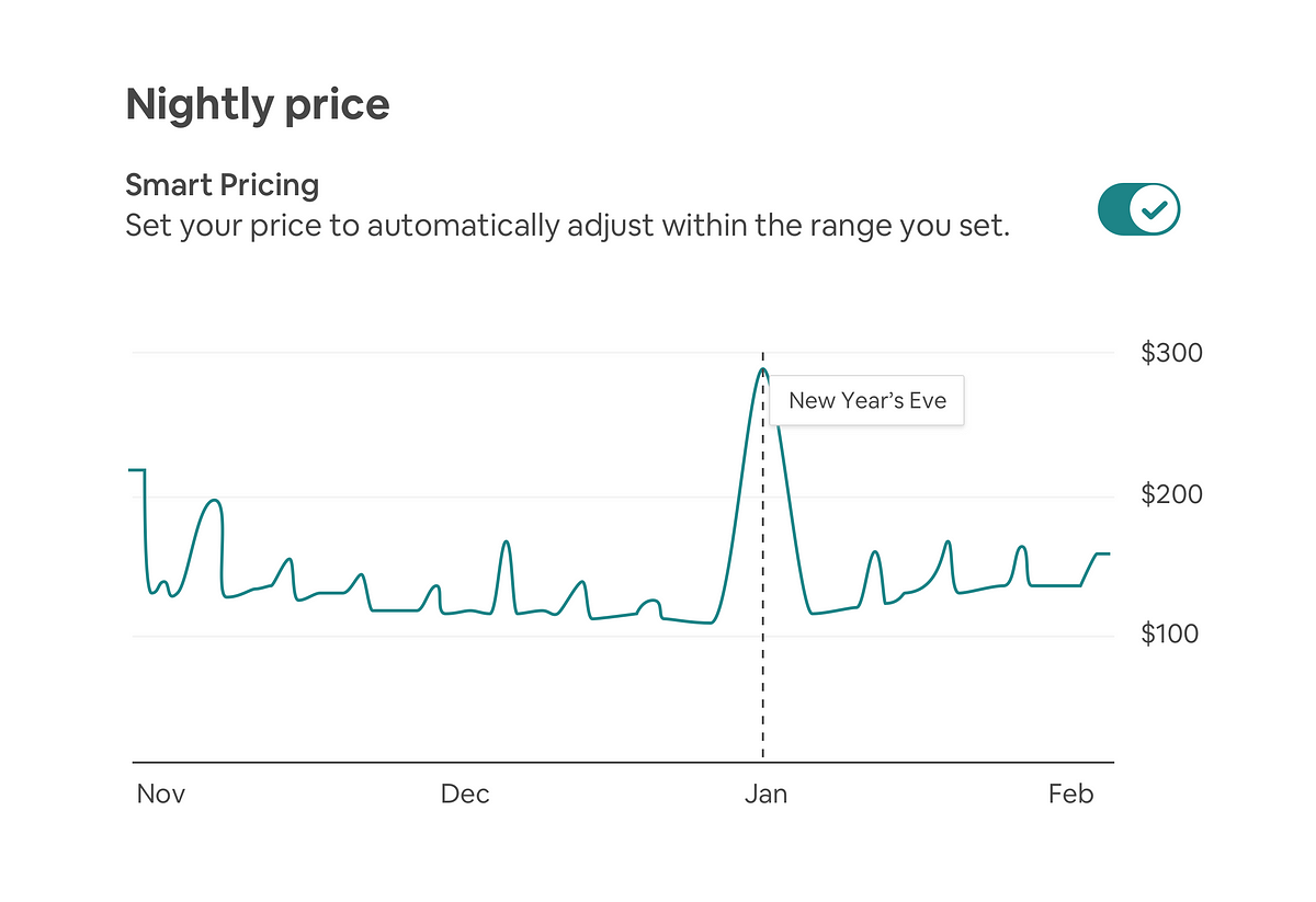
Learning the booking lead time distribution helps power our pricing system. Airbnb launched Smart Pricing to help hosts set optimal prices and maximize earnings. These tools take into account factors like demand, supply and individual listing properties in order to make price suggestions for all check-in dates on the calendar. However, market conditions typically change as booking dates get closer to check-in dates, and, as a result, it is critical for us to account for these changes and help hosts keep their prices optimized for market conditions.

As an example, on a high demand night like New Year’s Eve, guests tend to book more in advance (i.e. at long lead times) than at other times of the year. This information helps set the right prices for New Year’s Eve. Similarly, locations play a big part in this too. A supply-constrained market gets bookings well ahead of check-ins compared to a holiday market like South Beach, Miami. By learning the arrival process for every check-in date and location, Smart Pricing accounts for this “early demand” and generates a pricing policy that allows hosts to optimally update their prices as we approach check-in.

What Does the Arrival Process Look Like?

To make the problem more concrete, let’s start by introducing some notation. Let X_T(t) = P( Xijt=1 | Bij = 1) represent the lead time distribution of guest bookings, where

• T is a random variable representing lead time
• i be check-in date
• j be a listing of interest
• Bij be 1 if the check-in day ended up getting booked
• Xijt be 1 if the check-in day was booked at lead time

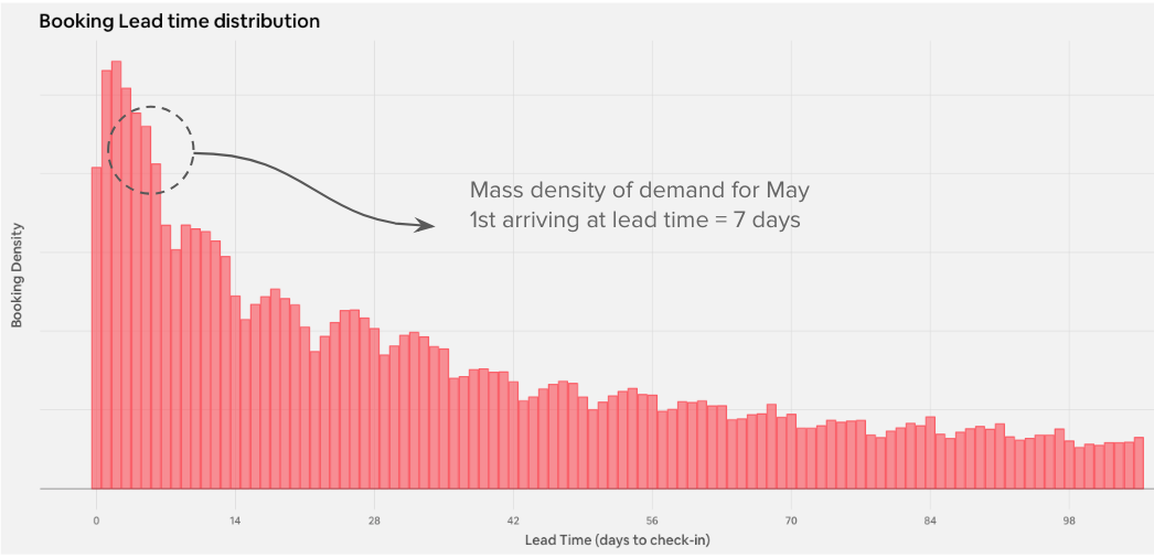
The figure below is an example of the lead time distribution aggregated to a market level. As we can see, the booking mass density gradually increases as we approach check-in (right to left), since guests don’t always plan their trips well in advance.

Our goal is to learn and estimate f (the density of the distribution above), for each listing i, check-in date j, and every lead day t heading into check-in.

Can We Use Machine Learning Directly?

What would using a typical ML approach look like for this problem? Well, we would first build out training dataset with relevant features X and labels Y. In our case, the label would be the lead time for every guest booking. To predict this label, Airbnb has accumulated various predictor signals that capture market supply, market demand, as well as listing-level features. The model would then predict the average lead time for each check-in date. However, in the end, we concluded that an ML approach would have several complications:

• Accounting for probabilistic outcomes: The arrival process is stochastic. For the purposes of optimal pricing, we need to know the distribution of bookings over lead time and not just the average lead time to book.
• Sparsity: Every listing gets booked at most once for a check-in date, leading to a highly sparse data set that would be challenging to handle without adding significant model complexity We will have to architect the model in a way that pools listing information together, enabling transfer learning across listings.
• High dimensionality: At Airbnb, we have millions of unique listings — each with its own defining characteristics and features that govern the arrival process. This makes every listing a very high dimensional data point and inefficient to use in a classic ML framework.
• Scale: The model will need to make predictions along three dimensions, ie. the triplet of (listings x check-in x number of lead times). This comes at a O(10⁶ x 10² x 10³) complexity, requiring very large training and scoring data sets and risks poor latency.

In addition to these challenges, close examination of the lead time distribution revealed a distinct structure of unimodal distribution with clear cyclical patterns (likely weekday/weekend movements) — in fact, taking a closer look, we noticed that the distributions resembled a generalized exponential family. Considering these strong parametric characteristics along with the complexities of an ML-only approach we were inspired to try a hybrid approach combining ML and structural modeling.

Machine Learning vs Structural Modeling, or Both?

Modern ML models fare very well in terms of predictive performance, but seldom model the underlying data generation mechanism. In contrast, structural models provide interpretability by allowing us to explicitly specify the relationships between the variables (features and responses) to reflect the process that gives rise to the data, but often fall short on predictive performance. Combining the two schools of thought allows us to exploit the strengths of each approach to better model the data generating process as well as achieve good model performance.

When we have good intuition for a modeling task, we can use our insights to reinforce an ML model with structural context. Imagine we are looking to predict a response Y based on features (X₀,…,Xn). Ordinarily, we would train our favorite ML model to predict. However, suppose we also know that Y is distributed over an input feature X₀ with a distribution F parameterized by ? i.e. Y~ F(X₀; ? ), we could leverage this information and decompose the task to learning ? using features (X₀,…,Xn), and then simply plug our estimate of ? back into f to arrive at Y in the final step.

By employing this hybrid approach, we can leverage both the algorithmic powerhouse that ML provides and the informed intuition of statistical modeling. This is the approach we took to model lead time dynamics.

The Modeling Methodology

1. Laying the Foundation — Generating Demand Aggregations

As a first step, we start by pooling our supply to form listing clusters. The clustering is learned using guest search patterns on Airbnb, with each cluster mapped to a common set of guest preferences. As a result, the listings within a cluster share common demand profiles and tend to witness similar lead time distributions. This process helps overcome problems of dimensionality and scale.

Unlike commoditized accommodations in the hotel industry, every listing on Airbnb is unique. Airbnb homes span over a broad spectrum, from price, location, quality, to size, etc. This vast heterogeneity brings challenges for personalization. It’s challenging to estimate the arrival process for every listing and every check-in date separately. Clustering listings into “demand aggregations” addresses this challenge. A demand aggregation refers to a cluster of listings that share common demand profiles.

When guests come to Airbnb, they browse through multiple listings in our catalogue and potentially choose one to book. By tracing a guest’s path to purchase, we learn more about their considerations and preferences. When two listings frequently co-appear in the purchase path of several guests, they tend to mirror a common set of guest preferences. For example, listings in west lake Tahoe often co-appear in search sessions of ski enthusiasts looking to stay at Airbnb (picture below).

We can employ the notion above to generate low dimensional listing embeddings, similar to this embedding technique. This work produces listing embeddings which semantically relate to their demand profiles. With the listing embeddings at hand, we then clustered them together hierarchically to form demand aggregations. Each demand aggregation represents a consideration set that guests browsed over when making a booking. Such a framework is quite common in discrete choice models for demand estimation, specially online marketplaces. Here are some visuals of how these clusters might looks like.