
二分類模型評價指標-Sklearn
阿新 • • 發佈:2018-12-30
Sklearn的metrics模組下有多個計算模型評價指標的函式,本文只介紹二分類的指標函式。
1.準確率
1.1引數說明
sklearn.metrics.accuracy_score(y_true, y_pred, normalize=True, sample_weight=None)| 解釋 | |
|---|---|
| 引數 |
y_true 真實的label,一維陣列格式 2.y_pred 模型預測的label,一維陣列 3.normalize 預設True,返回正確預測的比例,False返回預測正確的個數 4.sample_weight 樣本權重 |
| 返回結果 | score:返回正確的比例或者個數,由normalize指定 |
1.2 應用
import pandas as pd
import numpy as np
from sklearn import metrics
y_pred = [0,1,0,1]
y_true = [0,0,0,0]
## 返回正確率
metrics.accuracy_score(y_pred,y_true)0.5
## 返回正確個數
metrics.accuracy_score(y_pred,y_true,normalize=False 2
2.混淆矩陣
2.1 引數說明
| 引數 |
y_true 真實的label,一維陣列格式,列名 2.y_pred 模型預測的label,一維陣列,行名 3.labels 預設不指定,此時y_true、y_pred取並集,升序,做label 4.sample_weight 樣本權重 |
| 返回結果 | C:返回混淆矩陣,注意label |
2.2 應用
y_true = [2, 0, 2, 0, 0, 1]
y_pred = [0, 0, 2, 2, 3, 2]
metrics.confusion_matrix(y_true, y_pred)
array([[1, 0, 1, 1], [0, 0, 1, 0], [1, 0, 1, 0], [0, 0, 0, 0]], dtype=int64)
import itertools
import numpy as np
import matplotlib.pyplot as plt
from sklearn import svm, datasets
from sklearn.model_selection import train_test_split
from sklearn.metrics import confusion_matrix

def plot_confusion_matrix(cm, classes,
                          normalize=False,
                          title='Confusion matrix',
                          cmap=plt.cm.Blues):
    """
    This function prints and plots the confusion matrix.
    Normalization can be applied by setting `normalize=True`.
    """
    if normalize:
        cm = cm.astype('float') / cm.sum(axis=1)[:, np.newaxis]
        print("Normalized confusion matrix")
    else:
        print('Confusion matrix, without normalization')

    print(cm)

    plt.imshow(cm, interpolation='nearest', cmap=cmap)
    plt.title(title)
    plt.colorbar()
    tick_marks = np.arange(len(classes))
    plt.xticks(tick_marks, classes, rotation=45)
    plt.yticks(tick_marks, classes)

    fmt = '.2f' if normalize else 'd'
    thresh = cm.max() / 2.
    for i, j in itertools.product(range(cm.shape[0]), range(cm.shape[1])):
        plt.text(j, i, format(cm[i, j], fmt),
                 horizontalalignment="center",
                 color="white" if cm[i, j] > thresh else "black")

    plt.ylabel('True label')
    plt.xlabel('Predicted label')
    plt.tight_layout()
y_test = [1, 1, 1, 0]
y_pred = [1, 1, 0, 0]
# Compute confusion matrix
# #注意混淆矩陣要求預測結果在第一個位置
cnf_matrix = confusion_matrix(y_test, y_pred)
## 限制兩位小數
np.set_printoptions(precision=2)# Plot non-normalized confusion matrix
plt.figure()
plot_confusion_matrix(cnf_matrix, classes=[0, 1], title='Confusion matrix, without normalization')
plt.show()Confusion matrix, without normalization
[[1 0]
[1 2]]

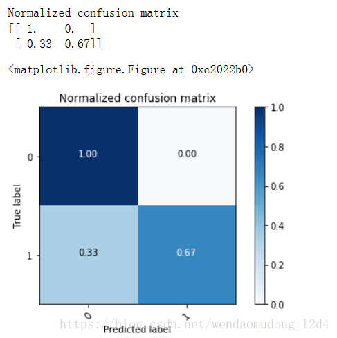
# Plot normalized confusion matrix
plt.figure()
plot_confusion_matrix(
    cnf_matrix,
    classes=[0, 1],
    normalize=True,
    title='Normalized confusion matrix')

plt.show()
Normalized confusion matrix
[[ 1. 0. ]
[ 0.33 0.67]]
<matplotlib.figure.Figure at 0xc2022b0>
3. Recall&Precision
3.1 引數說明
| 引數 |
y_true 真實的label,一維陣列格式,列名 2.y_pred 模型預測的label,一維陣列,行名 3.labels 預設不指定,此時y_true、y_pred取並集,升序,做label 4.sample_weight 樣本權重 5.target_names 行標籤,順序和label的要一致 6.digits int,小數的位數 7. output_dict 輸出格式,預設False,如果True,返回字典 |
| 返回結果 | report:返回計算結果,形式依賴於output_dict |
3.2 應用
要注意y_true和y_pred的位置順序。
y_true = [0, 1, 2, 2, 2]
y_pred = [0, 0, 2, 2, 1]
target_names = ['class 0', 'class 1', 'class 2']
print(metrics.classification_report(y_true, y_pred))
precision recall f1-score support
0 0.50 1.00 0.67 1
1 0.00 0.00 0.00 1
2 1.00 0.67 0.80 3
avg / total 0.70 0.60 0.61 5
print(metrics.classification_report(y_true, y_pred, target_names=target_names)) precision recall f1-score support
class 0 0.50 1.00 0.67 1
class 1 0.00 0.00 0.00 1
class 2 1.00 0.67 0.80 3
avg / total 0.70 0.60 0.61 5
4.Roc&Auc
計算AUC,畫ROC曲線的貌似沒有直接的函式。
4.1 引數
| 引數 |
y_true 真實的label,一維陣列格式,列名 2.y_pred 模型預測的label,一維陣列,行名 3.average 有多個引數可選,一般預設即可 4.sample_weight 樣本權重 5.max_fpr 取值範圍[0,1),如果不是None,則會標準化,使得最大值=max_fpr |
| 返回結果 | report:返回計算結果,形式依賴於output_dict |
y_true = np.array([0, 0, 1, 1])
y_scores = np.array([0.1, 0.4, 0.35, 0.8])
metrics.roc_auc_score(y_true, y_scores)
0.75
2018-07-16 於南京市建鄴區新城科技園