
yolov3 pytorch實現1
yolo不多做介紹,請參相關部落格和論文
本文主要是使用pytorch來對yolo中每一步進行實現 參考:https://blog.paperspace.com/tag/series-yolo/
需要了解:
- 卷積神經網路原理及pytorch實現
- yolo等目標檢測演算法的檢測原理,相關概念如 anchor(錨點)、ROI(感興趣區域)、IOU(交併比)、NMS(非極大值抑制)、LR softmax分類、邊框迴歸等
本文主要分為四個部分:
- yolo網路層級的定義
- 向前傳播
- 置信度閾值和非極大值抑制
- 輸入和輸出流程
yolo網路層級的定義
Darknet 是 yolo 對目標特徵提取的框架,從yolov1的darknet 到 v2,v3的darknet-19,darknet-53


可以看到yolov3的時候已經沒有全連線層了,最後只有一個池化層,還加入了resnet的機制。
Demo
layer     filters    size              input                output
    0 conv     32  3 x 3 / 1   416 x 416 x   3   ->   416 x 416 x  32  0.299 BFLOPs
    1 conv     64  3 x 3 / 2   416 x 416 x  32   ->   208 x 208 x  64  1.595 BFLOPs
    2 conv     32  1 x 1 / 1   208 x 208 x  64   ->   208 x 208 x  32  0.177 BFLOPs
    3 conv     64  3 x 3 / 1   208 x 208 x  32   ->   208 x 208 x  64  1.595 BFLOPs
    4 res    1                 208 x 208 x  64   ->   208 x 208 x  64
    5 conv    128  3 x 3 / 2   208 x 208 x  64   ->   104 x 104 x 128  1.595 BFLOPs
    6 conv     64  1 x 1 / 1   104 x 104 x 128   ->   104 x 104 x  64  0.177 BFLOPs
    7 conv    128  3 x 3 / 1   104 x 104 x  64   ->   104 x 104 x 128  1.595 BFLOPs
    8 res    5                 104 x 104 x 128   ->   104 x 104 x 128
    9 conv     64  1 x 1 / 1   104 x 104 x 128   ->   104 x 104 x  64  0.177 BFLOPs
   10 conv    128  3 x 3 / 1   104 x 104 x  64   ->   104 x 104 x 128  1.595 BFLOPs
   11 res    8                 104 x 104 x 128   ->   104 x 104 x 128
   12 conv    256  3 x 3 / 2   104 x 104 x 128   ->    52 x  52 x 256  1.595 BFLOPs
   13 conv    128  1 x 1 / 1    52 x  52 x 256   ->    52 x  52 x 128  0.177 BFLOPs
   14 conv    256  3 x 3 / 1    52 x  52 x 128   ->    52 x  52 x 256  1.595 BFLOPs
   15 res   12                  52 x  52 x 256   ->    52 x  52 x 256
   16 conv    128  1 x 1 / 1    52 x  52 x 256   ->    52 x  52 x 128  0.177 BFLOPs
   17 conv    256  3 x 3 / 1    52 x  52 x 128   ->    52 x  52 x 256  1.595 BFLOPs
   18 res   15                  52 x  52 x 256   ->    52 x  52 x 256
   19 conv    128  1 x 1 / 1    52 x  52 x 256   ->    52 x  52 x 128  0.177 BFLOPs
   20 conv    256  3 x 3 / 1    52 x  52 x 128   ->    52 x  52 x 256  1.595 BFLOPs
   21 res   18                  52 x  52 x 256   ->    52 x  52 x 256
   22 conv    128  1 x 1 / 1    52 x  52 x 256   ->    52 x  52 x 128  0.177 BFLOPs
   23 conv    256  3 x 3 / 1    52 x  52 x 128   ->    52 x  52 x 256  1.595 BFLOPs
   24 res   21                  52 x  52 x 256   ->    52 x  52 x 256
   25 conv    128  1 x 1 / 1    52 x  52 x 256   ->    52 x  52 x 128  0.177 BFLOPs
   26 conv    256  3 x 3 / 1    52 x  52 x 128   ->    52 x  52 x 256  1.595 BFLOPs
   27 res   24                  52 x  52 x 256   ->    52 x  52 x 256
   28 conv    128  1 x 1 / 1    52 x  52 x 256   ->    52 x  52 x 128  0.177 BFLOPs
   29 conv    256  3 x 3 / 1    52 x  52 x 128   ->    52 x  52 x 256  1.595 BFLOPs
   30 res   27                  52 x  52 x 256   ->    52 x  52 x 256
   31 conv    128  1 x 1 / 1    52 x  52 x 256   ->    52 x  52 x 128  0.177 BFLOPs
   32 conv    256  3 x 3 / 1    52 x  52 x 128   ->    52 x  52 x 256  1.595 BFLOPs
   33 res   30                  52 x  52 x 256   ->    52 x  52 x 256
   34 conv    128  1 x 1 / 1    52 x  52 x 256   ->    52 x  52 x 128  0.177 BFLOPs
   35 conv    256  3 x 3 / 1    52 x  52 x 128   ->    52 x  52 x 256  1.595 BFLOPs
   36 res   33                  52 x  52 x 256   ->    52 x  52 x 256
   37 conv    512  3 x 3 / 2    52 x  52 x 256   ->    26 x  26 x 512  1.595 BFLOPs
   38 conv    256  1 x 1 / 1    26 x  26 x 512   ->    26 x  26 x 256  0.177 BFLOPs
   39 conv    512  3 x 3 / 1    26 x  26 x 256   ->    26 x  26 x 512  1.595 BFLOPs
   40 res   37                  26 x  26 x 512   ->    26 x  26 x 512
   41 conv    256  1 x 1 / 1    26 x  26 x 512   ->    26 x  26 x 256  0.177 BFLOPs
   42 conv    512  3 x 3 / 1    26 x  26 x 256   ->    26 x  26 x 512  1.595 BFLOPs
   43 res   40                  26 x  26 x 512   ->    26 x  26 x 512
   44 conv    256  1 x 1 / 1    26 x  26 x 512   ->    26 x  26 x 256  0.177 BFLOPs
   45 conv    512  3 x 3 / 1    26 x  26 x 256   ->    26 x  26 x 512  1.595 BFLOPs
   46 res   43                  26 x  26 x 512   ->    26 x  26 x 512
   47 conv    256  1 x 1 / 1    26 x  26 x 512   ->    26 x  26 x 256  0.177 BFLOPs
   48 conv    512  3 x 3 / 1    26 x  26 x 256   ->    26 x  26 x 512  1.595 BFLOPs
   49 res   46                  26 x  26 x 512   ->    26 x  26 x 512
   50 conv    256  1 x 1 / 1    26 x  26 x 512   ->    26 x  26 x 256  0.177 BFLOPs
   51 conv    512  3 x 3 / 1    26 x  26 x 256   ->    26 x  26 x 512  1.595 BFLOPs
   52 res   49                  26 x  26 x 512   ->    26 x  26 x 512
   53 conv    256  1 x 1 / 1    26 x  26 x 512   ->    26 x  26 x 256  0.177 BFLOPs
   54 conv    512  3 x 3 / 1    26 x  26 x 256   ->    26 x  26 x 512  1.595 BFLOPs
   55 res   52                  26 x  26 x 512   ->    26 x  26 x 512
   56 conv    256  1 x 1 / 1    26 x  26 x 512   ->    26 x  26 x 256  0.177 BFLOPs
   57 conv    512  3 x 3 / 1    26 x  26 x 256   ->    26 x  26 x 512  1.595 BFLOPs
   58 res   55                  26 x  26 x 512   ->    26 x  26 x 512
   59 conv    256  1 x 1 / 1    26 x  26 x 512   ->    26 x  26 x 256  0.177 BFLOPs
   60 conv    512  3 x 3 / 1    26 x  26 x 256   ->    26 x  26 x 512  1.595 BFLOPs
   61 res   58                  26 x  26 x 512   ->    26 x  26 x 512
   62 conv   1024  3 x 3 / 2    26 x  26 x 512   ->    13 x  13 x1024  1.595 BFLOPs
   63 conv    512  1 x 1 / 1    13 x  13 x1024   ->    13 x  13 x 512  0.177 BFLOPs
   64 conv   1024  3 x 3 / 1    13 x  13 x 512   ->    13 x  13 x1024  1.595 BFLOPs
   65 res   62                  13 x  13 x1024   ->    13 x  13 x1024
   66 conv    512  1 x 1 / 1    13 x  13 x1024   ->    13 x  13 x 512  0.177 BFLOPs
   67 conv   1024  3 x 3 / 1    13 x  13 x 512   ->    13 x  13 x1024  1.595 BFLOPs
   68 res   65                  13 x  13 x1024   ->    13 x  13 x1024
   69 conv    512  1 x 1 / 1    13 x  13 x1024   ->    13 x  13 x 512  0.177 BFLOPs
   70 conv   1024  3 x 3 / 1    13 x  13 x 512   ->    13 x  13 x1024  1.595 BFLOPs
   71 res   68                  13 x  13 x1024   ->    13 x  13 x1024
   72 conv    512  1 x 1 / 1    13 x  13 x1024   ->    13 x  13 x 512  0.177 BFLOPs
   73 conv   1024  3 x 3 / 1    13 x  13 x 512   ->    13 x  13 x1024  1.595 BFLOPs
   74 res   71                  13 x  13 x1024   ->    13 x  13 x1024
   75 conv    512  1 x 1 / 1    13 x  13 x1024   ->    13 x  13 x 512  0.177 BFLOPs
   76 conv   1024  3 x 3 / 1    13 x  13 x 512   ->    13 x  13 x1024  1.595 BFLOPs
   77 conv    512  1 x 1 / 1    13 x  13 x1024   ->    13 x  13 x 512  0.177 BFLOPs
   78 conv   1024  3 x 3 / 1    13 x  13 x 512   ->    13 x  13 x1024  1.595 BFLOPs
   79 conv    512  1 x 1 / 1    13 x  13 x1024   ->    13 x  13 x 512  0.177 BFLOPs
   80 conv   1024  3 x 3 / 1    13 x  13 x 512   ->    13 x  13 x1024  1.595 BFLOPs
   81 conv    255  1 x 1 / 1    13 x  13 x1024   ->    13 x  13 x 255  0.088 BFLOPs
   82 detection
   83 route  79
   84 conv    256  1 x 1 / 1    13 x  13 x 512   ->    13 x  13 x 256  0.044 BFLOPs
   85 upsample            2x    13 x  13 x 256   ->    26 x  26 x 256
   86 route  85 61
   87 conv    256  1 x 1 / 1    26 x  26 x 768   ->    26 x  26 x 256  0.266 BFLOPs
   88 conv    512  3 x 3 / 1    26 x  26 x 256   ->    26 x  26 x 512  1.595 BFLOPs
   89 conv    256  1 x 1 / 1    26 x  26 x 512   ->    26 x  26 x 256  0.177 BFLOPs
   90 conv    512  3 x 3 / 1    26 x  26 x 256   ->    26 x  26 x 512  1.595 BFLOPs
   91 conv    256  1 x 1 / 1    26 x  26 x 512   ->    26 x  26 x 256  0.177 BFLOPs
   92 conv    512  3 x 3 / 1    26 x  26 x 256   ->    26 x  26 x 512  1.595 BFLOPs
   93 conv    255  1 x 1 / 1    26 x  26 x 512   ->    26 x  26 x 255  0.177 BFLOPs
   94 detection
   95 route  91
   96 conv    128  1 x 1 / 1    26 x  26 x 256   ->    26 x  26 x 128  0.044 BFLOPs
   97 upsample            2x    26 x  26 x 128   ->    52 x  52 x 128
   98 route  97 36
   99 conv    128  1 x 1 / 1    52 x  52 x 384   ->    52 x  52 x 128  0.266 BFLOPs
  100 conv    256  3 x 3 / 1    52 x  52 x 128   ->    52 x  52 x 256  1.595 BFLOPs
  101 conv    128  1 x 1 / 1    52 x  52 x 256   ->    52 x  52 x 128  0.177 BFLOPs
  102 conv    256  3 x 3 / 1    52 x  52 x 128   ->    52 x  52 x 256  1.595 BFLOPs
  103 conv    128  1 x 1 / 1    52 x  52 x 256   ->    52 x  52 x 128  0.177 BFLOPs
  104 conv    256  3 x 3 / 1    52 x  52 x 128   ->    52 x  52 x 256  1.595 BFLOPs
  105 conv    255  1 x 1 / 1    52 x  52 x 256   ->    52 x  52 x 255  0.353 BFLOPs
  106 detection
1.具體效能比較暫不多提,實現方法如下:
darknet 網路的 config 從官網中可以下載: https://pjreddie.com/darknet/yolo/
每個config包含如下一些模組:
1.1.卷積網路模型,步長有1、2。步長為2做上取樣

1.2.yolo3中shortcut 類似於resnet,跨通道連線,

1.3.route層。當層級有兩個值時,它將返回由這兩個值索引的拼接特徵圖。實驗中為-1 和 61,因此該層級將輸出從前一層級(-1)到第 61 層的特徵圖,並將它們按深度拼接。最後檢測時像FPN中對不同層次的特徵一個結合,更好檢測小目標
1. 4.上取樣層

1.5.net網路訓練的引數層

1.6.yolo層,設定一些引數,anchor的尺寸是由k-means聚類得到的

所以我們要解析config檔案來構建我們的網路。首先建立darknet.py 檔案(讀取的是yolo3的darknet-53)
from __future__ import division

import torch
import torch.nn as nn
import torch.nn.functional as F
from torch.autograd import Variable
import numpy as np

def parse_cfg(cfgfile):
    #解析cfg,將每個塊儲存為詞典(鍵 值),然後新增到列表blocks中
    file = open(cfgfile, 'r')
    lines = file.read().split('\n') #按行儲存
    lines = [x for x in lines if len(x) > 0] #不讀空行
    lines = [x for x in lines if x[0] != '#'] #不讀註釋
    lines = [x.rstrip().lstrip() for x in lines]#去除邊緣空白
    #遍歷列表 得到塊
    block = {}
    blocks = []

    for line in lines:
        if line[0] == '[': #起始mark 標記
            if len(block) != 0: #判斷是否為空
                blocks.append(block)
                block = {} #重新初始化block
            block["type"] = line[1:-1].rstrip()
        else:
            key, value = line.split('=')
            block[key.rstrip()] = value.lstrip()
    blocks.append(block)
    print(blocks)
    return blocks
blocks 是以字典的形式儲存資訊,輸出為:
{'type': 'convolutional', 'batch_normalize': '1', 'filters': '32', 'size': '3', 'stride': '1', 'pad': '1', 'activation': 'leaky'}, {'type': 'convolutional', 'batch_normalize': '1', 'filters': '64', 'size': '3', 'stride': '2', 'pad': '1', 'activation': 'leaky'},
{'type': 'shortcut', 'from': '-3', 'activation': 'linear'},
{'type': 'route', 'layers': '-4'},
{'type': 'upsample', 'stride': '2'},
{'type': 'net', 'batch': '1', 'subdivisions': '1', 'width': '416', 'height': '416', 'channels': '3', 'momentum': '0.9', 'decay': '0.0005', 'angle': '0', 'saturation': '1.5', 'exposure': '1.5', 'hue': '.1', 'learning_rate': '0.001', 'burn_in': '1000', 'max_batches': '500200', 'policy': 'steps', 'steps': '400000,450000', 'scales': '.1,.1'},
{'type': 'yolo', 'mask': '0,1,2', 'anchors': '10,13, 16,30, 33,23, 30,61, 62,45, 59,119, 116,90, 156,198, 373,326', 'classes': '80', 'num': '9', 'jitter': '.3', 'ignore_thresh': '.5', 'truth_thresh': '1', 'random': '1'},
然後利用字典中的資訊構建網路層:
def create_modules(blocks):
    net_info = blocks[0]#儲存網路資訊
    module_list = nn.ModuleList()
    prev_fileters = 3 #初始化影象通道   但是卷積深度由上一層決定
    output_filters =[]#追蹤之前的層用來路由

    #讀取bloks中的元素
    for index, x in enumerate(blocks[1:]):
        module = nn.Sequential()

        #讀取convolutional塊中的資訊
        if (x['type'] == 'convolutional'):
            activation = x['activation']
            try:
                batch_normalize = int(x["batch_normalize"])
                bias = False
            except:
                batch_normalize = 0
                bias = True

            filters = int(x["filters"]) #卷積核數量(維度)
            padding = int(x["pad"]) #邊框填補
            kernel_size = int(x["size"]) #卷積核大小
            stride = int(x["stride"]) #步長

            if padding:
                pad = (kernel_size - 1)//2
            else:
                pad = 0
###
            conv = nn.Conv2d(prev_fileters,filters,kernel_size,
                             stride,pad,bias=bias)
            module.add_module("conv_{0}".format(index),conv)

            if batch_normalize:
                bn = nn.BatchNorm2d(filters)
                module.add_module("batch_norm_{0}".format(index),bn)

            if activation == "leaky":
                activn = nn.LeakyReLU(0.1,inplace=True)
                module.add_module("leaky_{0}".format(index),activn)
###
        #讀取上取樣塊
        elif (x["type"] == "upsample"):
            stride = int(x["stride"])
            upsample = nn.Upsample(scale_factor=2, mode="nearest")
            module.add_module("upsample_{}".format(index),upsample)

        #讀取路由塊
        elif (x["type"] == "route"):
            x["layers"] = x["layers"].split(',')
            start = int(x["layers"][0])
            try:
                end = int(x["layers"][1])
            except:
                end = 0

            if start > 0:
                start = start - index
            if end > 0:
                end = end - index
            route = EmptyLayer()
            module.add_module("route_{0}".format(index),route)
            if end < 0:
                filters = output_filters[index + start] + output_filters[index + end]
            else:
                filters = output_filters[index + start]

        #讀取shortcut
        elif x["type"] == "shortcut":
            shortcut = EmptyLayer()
            module.add_module("shortcut_{}".format(index),shortcut)

        #讀取yolo
        elif x["type"] == "yolo":
            mask = x["mask"].split(",")
            mask = [int(x) for x in mask]
            #讀取anchor的尺寸
            anchors = x["anchors"].split(",")
            anchors = [int(a) for a in anchors]
            anchors = [(anchors[i], anchors[i+1]) for i in range(0, len(anchors),2)]
            anchors = [anchors[i] for i in mask]

            detection = DetectionLayer(anchors)
            module.add_module("Detection_{}".format(index),detection)

        module_list.append(module)
        prev_fileters = filters
        output_filters.append(filters)
    return (net_info, module_list)

blocks = parse_cfg("cfg/yolov3.cfg")
print(create_modules(blocks))
輸出:

其中,需在此之前定義兩個繼承nn.Module的類
class EmptyLayer(nn.Module):
    def __init__(self):
        super(EmptyLayer,self).__init__()

class DetectionLayer(nn.Module):
    def __init__(self, anchors):
        super(DetectionLayer, self).__init__()
        self.anchors = anchors
前向傳播
下一節介紹 然後根據讀取的網路資訊 定義一個前向傳播
首先定義一個nn.Module的類 Darknet,獲取blocks 和 module_list
class Darknet(nn.Module):
    def __init__(self, cfgfile):
        super(Darknet, self).__init__()
        self.blocks = parse_cfg(cfgfile)
        self.net_info, self.module_list = create_modules(self.blocks)
然後定義向前傳播
def forward(self, x, CUDA=False):
modules = self.blocks[1:]
outputs = {}
'''
write flag 表示我們是否遇到第一個檢測。如果 write 是 0,則收集器尚未初始化。
如果 write 是 1,則收集器已經初始化,我們只需要將檢測圖與收集器級聯起來即可。
'''
write = 0
#按順序讀modules 不同的層執行不同的操作
for i, module in enumerate(modules):
module_type = (module["type"])
if module_type == "convolutional" or module_type == "upsample":
x = self.module_list[i](x)
elif module_type == "route":
layers = module["layers"]
layers = [int(a) for a in layers]
if (layers[0]) > 0:
layers[0] = layers[0] - i
if len(layers) == 1:
x = outputs[i + (layers[0])]
else:
if (layers[1]) > 0:
layers[1] = layers[1] - i
map1 = outputs[i + layers[0]]
map2 = outputs[i + layers[1]]
x = t.cat((map1, map2), 1) #兩個張量(tensor)拼接在一起
elif module_type == "shortcut":
from_ = int(module["from"])
x = outputs[i-1] + outputs[i+from_]
#現在可以將三個不同尺度的檢測圖級聯成一個大的張量
elif module_type == "yolo":
anchors = self.module_list[i][0].anchors
inp_dim = int (self.net_info["height"])
num_classer = int (module["classes"])
x = x.data
x = predict_transform(x, inp_dim, anchors,
num_classer,CUDA)
if not write:
detections = x
write = 1
else:
detections = t.cat((detections, x), 1)
outputs[i] = x
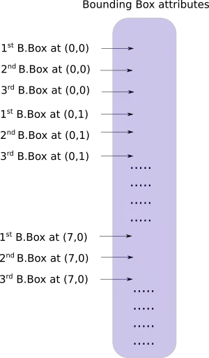
return detectionsYOLO 的輸出是一個卷積特徵圖,包含沿特徵圖深度的邊界框屬性。邊界框屬性由彼此堆疊的單元格預測得出。因此,如果你需要在 (5,6) 處訪問單元格的第二個邊框,那麼你需要通過 map[5,6, (5+C): 2*(5+C)] 將其編入索引。這種格式對於輸出處理過程(例如通過目標置信度進行閾值處理、新增對中心的網格偏移、應用錨點等)很不方便。
另一個問題是由於檢測是在三個尺度上進行的,預測圖的維度將是不同的。雖然三個特徵圖的維度不同,但對它們執行的輸出處理過程是相似的。如果能在單個張量而不是三個單獨張量上執行這些運算,就太好了。
為了解決這些問題,我們引入了函式 predict_transform 在utils.py檔案中
def predict_transform(prediction, inp_dim, anchors, num_classes, CUDA = True):


    batch_size = prediction.size(0)
    stride =  inp_dim // prediction.size(2)
    grid_size = inp_dim // stride
    bbox_attrs = 5 + num_classes
    num_anchors = len(anchors)

    prediction = prediction.view(batch_size, bbox_attrs*num_anchors, grid_size*grid_size)
    prediction = prediction.transpose(1,2).contiguous()
    prediction = prediction.view(batch_size, grid_size*grid_size*num_anchors, bbox_attrs)
    anchors = [(a[0]/stride, a[1]/stride) for a in anchors]

    #Sigmoid the  centre_X, centre_Y. and object confidencce
    prediction[:,:,0] = torch.sigmoid(prediction[:,:,0])
    prediction[:,:,1] = torch.sigmoid(prediction[:,:,1])
    prediction[:,:,4] = torch.sigmoid(prediction[:,:,4])

    #Add the center offsets
    grid = np.arange(grid_size)
    a,b = np.meshgrid(grid, grid)

    x_offset = torch.FloatTensor(a).view(-1,1)
    y_offset = torch.FloatTensor(b).view(-1,1)

    if CUDA:
        x_offset = x_offset.cuda()
        y_offset = y_offset.cuda()

    x_y_offset = torch.cat((x_offset, y_offset), 1).repeat(1,num_anchors).view(-1,2).unsqueeze(0)

    prediction[:,:,:2] += x_y_offset

    #log space transform height and the width
    anchors = torch.FloatTensor(anchors)

    if CUDA:
        anchors = anchors.cuda()

    anchors = anchors.repeat(grid_size*grid_size, 1).unsqueeze(0)
    prediction[:,:,2:4] = torch.exp(prediction[:,:,2:4])*anchors

    prediction[:,:,5: 5 + num_classes] = torch.sigmoid((prediction[:,:, 5 : 5 + num_classes]))

    prediction[:,:,:4] *= stride

    return prediction
predict_transform 函式把檢測特徵圖轉換成二維張量,張量的每一行對應邊界框的屬性,如下所示:
現在,在 darknet.py 檔案的頂部定義以下函式
def get_test_input():
    img = cv2.imread("dog-cycle-car.png")
    img = cv2.resize(img, (416,416))          #Resize to the input dimension
    img_ = img[:,:,::-1].transpose((2,0,1))  # BGR -> RGB | H X W C -> C X H X W
    img_ = img_[np.newaxis,:,:,:]/255.0       #Add a channel at 0 (for batch) | Normalise
    img_ = t.from_numpy(img_).float()     #Convert to float
    img_ = Variable(img_)                     # Convert to Variable
    return img_
測試程式碼
model = Darknet("cfg/yolov3.cfg")
inp = get_test_input()
pred = model(inp)
print (pred)
輸出

下載預訓練權重
https://pjreddie.com/media/files/yolov3.weights
讀取權重
    def load_weights(self, weightfile):
        fp = open(weightfile, "rb")

        header = np.fromfile(fp, dtype = np.int32, count = 5)
        self.header = t.from_numpy(header)
        self.seen = self.header[3]

        weights = np.fromfile(fp, dtype=np.float32)

        ptr = 0
        for i in range(len(self.module_list)):
            module_type = self.blocks[i+1]["type"]

            if module_type == "convolutional":
                module = self.module_list[i]
                try:
                    batch_normalize = int(self.blocks[i+1]["batch_normalize"])
                except:
                    batch_normalize = 0

                conv = module[0]

                if (batch_normalize):
                    bn = module[1]

                    num_bn_biases = bn.bias.numel()

                    bn_biases = t.from_numpy(weights[ptr:ptr + num_bn_biases])
                    ptr += num_bn_biases

                    bn_weights = t.from_numpy(weights[ptr: ptr + num_bn_biases])
                    ptr  += num_bn_biases

                    bn_running_mean = t.from_numpy(weights[ptr: ptr + num_bn_biases])
                    ptr += num_bn_biases

                    bn_running_var = t.from_numpy(weights[ptr: ptr + num_bn_biases])
                    ptr += num_bn_biases

                    #Cast the loaded weights into dims of model weights.
                    bn_biases = bn_biases.view_as(bn.bias.data)
                    bn_weights = bn_weights.view_as(bn.weight.data)
                    bn_running_mean = bn_running_mean.view_as(bn.running_mean)
                    bn_running_var = bn_running_var.view_as(bn.running_var)

                    #Copy the data to model
                    bn.bias.data.copy_(bn_biases)
                    bn.weight.data.copy_(bn_weights)
                    bn.running_mean.copy_(bn_running_mean)
                    bn.running_var.copy_(bn_running_var)

                else:
                    #Number of biases
                    num_biases = conv.bias.numel()

                    #Load the weights
                    conv_biases = t.from_numpy(weights[ptr: ptr + num_biases])
                    ptr = ptr + num_biases

                    #reshape the loaded weights according to the dims of the model weights
                    conv_biases = conv_biases.view_as(conv.bias.data)

                    #Finally copy the data
                    conv.bias.data.copy_(conv_biases)

                #Let us load the weights for the Convolutional layers
                num_weights = conv.weight.numel()

                #Do the same as above for weights
                conv_weights = t.from_numpy(weights[ptr:ptr+num_weights])
                ptr = ptr + num_weights

                conv_weights = conv_weights.view_as(conv.weight.data)
                conv.weight.data.copy_(conv_weights)
測試:
model = Darknet("cfg/yolov3.cfg")
model.load_weights("yolov3.weights")
inp = get_test_input()
pred = model(inp)
print (pred)
通過模型構建和權重載入,就可以開始進行目標檢測了
下一章介紹如何利用 objectness 置信度閾值和非極大值抑制生成最終的檢測結果。