CS231n assignment3 Q3 Network Visualization: Saliency maps, Class Visualization, and Fooling Images
阿新 • • 發佈:2019-01-05
Saliency Maps
一張saliency map告訴了我們在圖片中的每個畫素點對於這張圖片最後的預測得分的影響程度。為了計算它,我們要計算正確的那個類的未歸一化的打分對於圖片中每個畫素點的梯度。如果圖片的尺寸是(H,W,3),那麼梯度的尺寸也應該是(H,W,3);對於圖片中的每個畫素點,梯度值反映瞭如果某個畫素點的值改變一點點,分類的打分(score)會改變的程度大小。為了計算saliency map, 我們用梯度的絕對值,然後在3個channel上面求最大值,因此最後的saliency map的形狀應該是(H,W),並且所有的值都是非負數。
def compute_saliency_maps(X, y, model):
    """
    Compute a class saliency map using the model for images X and labels y.

    Input:
    - X: Input images, numpy array of shape (N, H, W, 3)
    - y: Labels for X, numpy of shape (N,)
    - model: A SqueezeNet model that will be used to compute the saliency map.

    Returns:
    - saliency: A numpy array of shape (N, H, W) giving the saliency maps for the
    input images.
    """
    saliency = None
    # Compute the score of the correct class for each example.
    # This gives a Tensor with shape [N], the number of examples.
    #
    # Note: this is equivalent to scores[np.arange(N), y] we used in NumPy
    # for computing vectorized losses.
    correct_scores = tf.gather_nd(model.scores,
                                  tf.stack((tf.range(X.shape[0]), model.labels), axis=1))
    ###############################################################################
    # TODO: Produce the saliency maps over a batch of images.                     #
    #                                                                             #
    # 1) Compute the “loss” using the correct scores tensor provided for you.     #
    #    (We'll combine losses across a batch by summing)                         #
    # 2) Use tf.gradients to compute the gradient of the loss with respect        #
    #    to the image (accessible via model.image).                               #
    # 3) Compute the actual value of the gradient by a call to sess.run().        #
    #    You will need to feed in values for the placeholders model.image and     #
    #    model.labels.                                                            #
    # 4) Finally, process the returned gradient to compute the saliency map.      #
    ###############################################################################
    #(1)(2) 分數對於輸入影象的梯度
    saliency_grad = tf.gradients(correct_scores,model.image)
    #(3) 運算求值
    saliency = sess.run(saliency_grad,feed_dict = {model.image:X,model.labels:y})[0]
    #(4) 處理
    saliency = np.absolute(saliency) #求絕對值
    saliency = np.amax(saliency,axis = -1) #求三個channel上最大的值
    ##############################################################################
    #                             END OF YOUR CODE                               #
    ##############################################################################
    return saliency

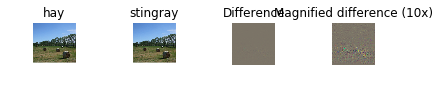
Fooling Images
我們也可以用影象梯度來生成一些”fooling images”,正如[3]中討論的那樣。 給定了一張圖片和一個目標的類,我們可以在圖片上做梯度上升來最大化目標類的分數,直到神經網路把這個圖片預測為目標類位置。
def make_fooling_image(X, target_y, model):
    """
    Generate a fooling image that is close to X, but that the model classifies
    as target_y.

    Inputs:
    - X: Input image, a numpy array of shape (1, 224, 224, 3)
    - target_y: An integer in the range [0, 1000)
    - model: Pretrained SqueezeNet model

    Returns:
    - X_fooling: An image that is close to X, but that is classifed as target_y
    by the model.
    """

    # Make a copy of the input that we will modify
    X_fooling = X.copy()

    # Step size for the update
    learning_rate = 1

    ##############################################################################
    # TODO: Generate a fooling image X_fooling that the model will classify as   #
    # the class target_y. Use gradient *ascent* on the target class score, using #
    # the model.scores Tensor to get the class scores for the model.image.   #
    # When computing an update step, first normalize the gradient:               #
    #   dX = learning_rate * g / ||g||_2                                         #
    #                                                                            #
    # You should write a training loop, where in each iteration, you make an     #
    # update to the input image X_fooling (don't modify X). The loop should      #
    # stop when the predicted class for the input is the same as target_y.       #
    #                                                                            #
    # HINT: It's good practice to define your TensorFlow graph operations        #
    # outside the loop, and then just make sess.run() calls in each iteration.   #
    #                                                                            #
    # HINT 2: For most examples, you should be able to generate a fooling image  #
    # in fewer than 100 iterations of gradient ascent. You can print your        #
    # progress over iterations to check your algorithm.                          #
    ##############################################################################
    score = model.scores[0, target_y]
    dX = tf.gradients(score, model.image)[0]
    dX = dX / tf.norm(dX)
    for i in range(100):
        ascent_step, scores = sess.run([dX, model.scores], feed_dict={model.image:X_fooling})
        if np.argmax(scores, axis=1) == target_y:
            break
        X_fooling += learning_rate * ascent_step
    ##############################################################################
    #                             END OF YOUR CODE                               #
    ##############################################################################
    return X_fooling
Class visualization
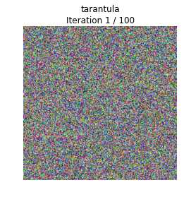
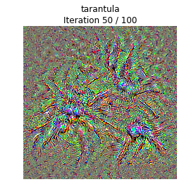
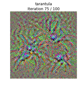
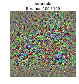
我們可以合成一張圖片來最大化一個特定類的打分;這可以給我們一些直觀感受,來看看模型在判斷圖片是當前這個類的時候它在關注的是圖片的哪些部分。
通過產生一個隨機噪聲的圖片,然後在目標類上做梯度上升,我們就可以生成一張模型會認為是目標類的圖片了。
def create_class_visualization(target_y, model, **kwargs):
    """
    Generate an image to maximize the score of target_y under a pretrained model.

    Inputs:
    - target_y: Integer in the range [0, 1000) giving the index of the class
    - model: A pretrained CNN that will be used to generate the image

    Keyword arguments:
    - l2_reg: Strength of L2 regularization on the image
    - learning_rate: How big of a step to take
    - num_iterations: How many iterations to use
    - blur_every: How often to blur the image as an implicit regularizer
    - max_jitter: How much to gjitter the image as an implicit regularizer
    - show_every: How often to show the intermediate result
    """
    l2_reg = kwargs.pop('l2_reg', 1e-3)
    learning_rate = kwargs.pop('learning_rate', 25)
    num_iterations = kwargs.pop('num_iterations', 100)
    blur_every = kwargs.pop('blur_every', 10)
    max_jitter = kwargs.pop('max_jitter', 16)
    show_every = kwargs.pop('show_every', 25)

    # We use a single image of random noise as a starting point
    X = 255 * np.random.rand(224, 224, 3)
    X = preprocess_image(X)[None]

    ########################################################################
    # TODO: Compute the loss and the gradient of the loss with respect to  #
    # the input image, model.image. We compute these outside the loop so   #
    # that we don't have to recompute the gradient graph at each iteration #
    #                                                                      #
    # Note: loss and grad should be TensorFlow Tensors, not numpy arrays!  #
    #                                                                      #
    # The loss is the score for the target label, target_y. You should     #
    # use model.scores to get the scores, and tf.gradients to compute  #
    # gradients. Don't forget the (subtracted) L2 regularization term!     #
    ########################################################################

    loss = None # scalar loss
    grad = None # gradient of loss with respect to model.image, same size as model.image
    pass
    loss = model.scores[0,target_y]
    grad = tf.gradients(loss,model.image)[0]
    grad -= 2*l2_reg*model.image
    ############################################################################
    #                             END OF YOUR CODE                             #
    ############################################################################


    for t in range(num_iterations):
        # Randomly jitter the image a bit; this gives slightly nicer results
        ox, oy = np.random.randint(-max_jitter, max_jitter+1, 2)
        X = np.roll(np.roll(X, ox, 1), oy, 2)

        ########################################################################
        # TODO: Use sess to compute the value of the gradient of the score for #
        # class target_y with respect to the pixels of the image, and make a   #
        # gradient step on the image using the learning rate. You should use   #
        # the grad variable you defined above.                                 #
        #                                                                      #
        # Be very careful about the signs of elements in your code.            #
        ########################################################################
        dX = sess.run(grad,feed_dict={model.image:X})
        X += learning_rate * dX
        ############################################################################
        #                             END OF YOUR CODE                             #
        ############################################################################

        # Undo the jitter
        X = np.roll(np.roll(X, -ox, 1), -oy, 2)

        # As a regularizer, clip and periodically blur
        X = np.clip(X, -SQUEEZENET_MEAN/SQUEEZENET_STD, (1.0 - SQUEEZENET_MEAN)/SQUEEZENET_STD)
        if t % blur_every == 0:
            X = blur_image(X, sigma=0.5)

        # Periodically show the image
        if t == 0 or (t + 1) % show_every == 0 or t == num_iterations - 1:
            plt.imshow(deprocess_image(X[0]))
            class_name = class_names[target_y]
            plt.title('%s\nIteration %d / %d' % (class_name, t + 1, num_iterations))
            plt.gcf().set_size_inches(4, 4)
            plt.axis('off')
            plt.show()
    return X