
統計學習方法邏輯斯蒂迴歸
邏輯斯諦迴歸(logistic regression) 是統計學習中的經典分類方法。 最大熵是概率模型學習的一個準則, 將其推廣到分類問題得到最大熵模型(maximum entropy model) 。邏輯斯諦迴歸模型與最大熵模型都屬於對數線性模型。本文只介紹邏輯斯諦迴歸。
設X是連續隨機變數, X服從Logistic distribution,
分佈函式: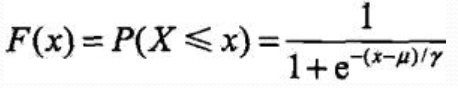
密度函式: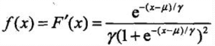
μ為位置引數, γ大於0為形狀引數, (μ,1/2)中心對稱

Sigmoid: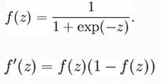


雙曲正切函式(tanh):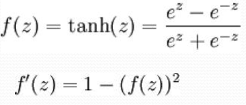

二項邏輯斯蒂迴歸
Binomial logistic regression model
由條件概率P(Y|X)表示的分類模型
形式化為logistic distribution
X取實數, Y取值1,0
事件的機率odds: 事件發生與事件不發生的概率之比為 稱為事件的發生比(the odds of experiencing an event),
對數機率:
對邏輯斯蒂迴歸:
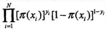
似然函式
logistic分類器是由一組權值係數組成的, 最關鍵的問題就是如何獲取這組權值, 通過極大似然函式估計獲得, 並且
Y~f(x;w)
似然函式是統計模型中引數的函式。 給定輸出x時, 關於引數θ的似然函式L(θ|x)(在數值上) 等於給定引數θ後變數X的概率: L(θ|x)=P(X=x|θ)
似然函式的重要性不是它的取值, 而是當引數變化時概率密度函式到底是變大還是變小。
極大似然函式: 似然函式取得最大值表示相應的引數能夠使得統計模型最為合理
那麼對於上述m個觀測事件, 設
其聯合概率密度函式, 即似然函式為:
目標: 求出使這一似然函式的值最大的引數估, w1,w2,…,wn,使得L(w)取得 最大值。
對L(w)取對數。
對數似然函式
對L(w)求極大值, 得到w的估計值。
通常採用梯度下降法及擬牛頓法, 學到的模型:
直接上程式碼吧,w的極大值採用梯度下降法,用的iris的資料集:
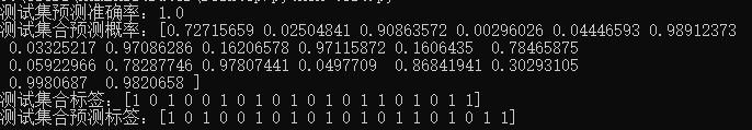
import numpy as np
import matplotlib.pyplot as plt
from sklearn.datasets import load_iris

class LogisticsRegression:

	def __init__(self):
		"""初始化Logistics Regression模型"""
		self.coef_ = None
		self.intercept_ = None
		self._theta = None

	def _sigmoid(self, t):
		return 1. / (1. + np.exp(-t))

	def accuracy_score(self, y_true, y_predict):
		"""計算y_true和y_predict之間的準確率"""
		assert len(y_true) == len(y_predict), \
			"the size of y_true must be equal to the size of y_predict"

		return np.sum(y_true == y_predict) / len(y_true)

	def fit(self, X_train, y_train, eta=0.01, n_iters=1e4):
		"""根據訓練資料集X_train, y_train, 使用梯度下降法訓練Logistics Regression模型"""
		assert X_train.shape[0] == y_train.shape[0], \
			"the size of X_train must be equal to the size of y_train"

		def J(theta, X_b, y):
			'''
			損失函式
			'''
			y_hat = self._sigmoid(X_b.dot(theta))
			try:
				return np.sum(y*np.log(y_hat) + (1-y)*np.log(1 - y_hat)) / len(y)
			except:
				return float('inf')

		def dJ(theta, X_b, y):
			'''
			求梯度
			'''
			return X_b.T.dot(self._sigmoid(X_b.dot(theta))  - y) / len(X_b)

		def gradient_descent(X_b, y, initial_theta, eta, n_iters=1e4, epsilon=1e-8):
			'''
			梯度下降
			'''
			theta = initial_theta
			cur_iter = 0
			while cur_iter < n_iters:
				gradient = dJ(theta, X_b, y)
				last_theta = theta
				theta = theta - eta * gradient
				if (abs(J(theta, X_b, y) - J(last_theta, X_b, y)) < epsilon):
					break
				cur_iter += 1
			return theta

		X_b = np.hstack([np.ones((len(X_train), 1)), X_train])
		initial_theta = np.zeros(X_b.shape[1])
		self._theta = gradient_descent(X_b, y_train, initial_theta, eta, n_iters)

		self.intercept_ = self._theta[0]
		self.coef_ = self._theta[1:]

		return self

	def predict_proba(self, X_predict):
		"""給定待預測資料集X_predict,返回表示X_predict的結果概率向量"""
		assert self.intercept_ is not None and self.coef_ is not None, \
			"must fit before predict!"
		assert X_predict.shape[1] == len(self.coef_), \
			"the feature number of X_predict must be equal to X_train"

		X_b = np.hstack([np.ones((len(X_predict), 1)), X_predict])
		return self._sigmoid(X_b.dot(self._theta))

	def predict(self, X_predict):
		"""給定待預測資料集X_predict,返回表示X_predict的結果向量"""
		assert self.intercept_ is not None and self.coef_ is not None, \
			"must fit before predict!"
		assert X_predict.shape[1] == len(self.coef_), \
			"the feature number of X_predict must be equal to X_train"
		proba = self.predict_proba(X_predict)
		return np.array(proba>=0.5, dtype = 'int')

	def score(self, X_test, y_test):
		"""根據測試資料集 X_test 和 y_test 確定當前模型的準確度"""

		y_predict = self.predict(X_test)
		return self.accuracy_score(y_test, y_predict)

	def __repr__(self):
		return "LogisticsRegression()"

iris = load_iris()

X = iris.data
y = iris.target

# 二項LogisticsRegression只適用二分類
X = X[y<2, :2]
y = y[y<2]

# # 畫出資料
# plt.scatter(X[y == 0, 0], X[y == 0, 1], color="red")
# plt.scatter(X[y == 1, 0], X[y == 1, 1], color="blue")
# plt.show()

def train_test_split(X, y, test_ratio=0.2, seed=None):
	"""將資料 X 和 y 按照test_ratio分割成X_train, X_test, y_train, y_test"""
	assert X.shape[0] == y.shape[0], \
		"the size of X must be equal to the size of y"
	assert 0.0 <= test_ratio <= 1.0, \
		"test_ration must be valid"

	if seed:
		np.random.seed(seed)

	shuffled_indexes = np.random.permutation(len(X))

	test_size = int(len(X) * test_ratio)
	test_indexes = shuffled_indexes[:test_size]
	train_indexes = shuffled_indexes[test_size:]

	X_train = X[train_indexes]
	y_train = y[train_indexes]

	X_test = X[test_indexes]
	y_test = y[test_indexes]

	return X_train, X_test, y_train, y_test

X_train, X_test, y_train, y_test = train_test_split(X, y, seed = 888)
log_reg = LogisticsRegression()
log_reg.fit(X_train, y_train)
print('測試集預測準確率:'+ str(log_reg.score(X_test, y_test)))
print('測試集合預測概率:'+ str(log_reg.predict_proba(X_test)))
print('測試集合標籤:'+ str(y_test))
print('測試集合預測標籤:' + str(log_reg.predict(X_test)))
結果:
多項logistic迴歸
設Y的取值集合為![]()
多項logistic迴歸模型