
Deep Learning 10_深度學習UFLDL教程:Convolution and Pooling_exercise(斯坦福大學深度學習教程)
前言
實驗環境:win7, matlab2015b,16G記憶體,2T機械硬碟
實驗內容:Exercise:Convolution and Pooling。從2000張64*64的RGB圖片(它是 the STL10 Dataset的一個子集)中提取特徵作為訓練資料集,訓練softmax分類器,然後從3200張64*64的RGB圖片(它是 the STL10 Dataset的另一個子集)中提取特徵作為測試資料集,輸入到前面已經訓練好的softmax分類器,把這3200張圖片分為4類:airplane, car, cat, dog。
實驗基礎說明:
1.怎麼樣從2000張64*64的RGB圖片中提取特徵得到訓練集,怎麼樣從3200張64*64的RGB圖片中提取特徵得到測試集?
因為這裡的RGB圖片是64*64,尺寸較大,而不是前面所有實驗中用的8*8的小影象塊,如果用Deep Learning九之深度學習UFLDL教程:linear decoder_exercise(斯坦福大學深度學習教程)中的方法直接從大尺寸圖片中提取特徵,那麼運算量就太大,所以,為了減小運算量,不能直接從大尺寸圖片中提取特徵,而是要用間接的減小運算量的方法,這個方法利用了自然影象的固有特性:自然影象的一部分的統計特性與其他部分是一樣的。這個固有特性也就意味著:從自然影象的某一部分A中學習的特徵L_feature也能用在該自然影象的另一部分B上。也就是說,對於這個自然影象上的所有位置,我們都能使用同樣的學習特徵。那麼究竟怎麼樣從這個大尺寸自然影象提取出它的L_feature特徵呢(這個特徵是從它的一部分A上學習到的)?答案是卷積!即把這個特徵和大尺寸圖片相卷,就可以提取這個大尺寸圖片的L_feature特徵,至於原因請看下面。這個L_feature特徵維數只會比大尺寸圖片稍微小一點(假設從小影象塊中學習到的特徵是8*8,大尺寸圖片是64*64,那麼這個L_feature特徵就是(64-8+1)*(64-8+1),即:57*57),如果把這些特徵作訓練資料集,那麼運算量還是很大,輸入層神經元節點數還是要57*57*3個,所以我們再對這些特徵用池化的方法(即:假設池化的維數是19,池化就是把57*57的特徵依次分為19*19的9個小部分,然後把每個小部分變為一個值(如果這個值是每個小部分的平均值就是平均池化,是最大值就是最大池化),從而把這個57*57的特徵變為了3*3的特徵),從而最後從2000張64*64的RGB圖片中提取出了3*3的特徵得到了訓練資料集,同理,可得到測試資料集。
具體方法:
①是從the STL10 Dataset中隨機抽樣選出10萬張8*8的RGB小影象塊(即:Sampled 8x8 patches from the STL-10 dataset),然後對它們進行預處理,具體包括:先對它們進行0均值化(注意:不是每個樣本各自單獨0均值化),再對它們進行ZCA白化。
②是對預處理後的資料利用線性解碼器提取出M個顏色特徵。
③是把2000張64*64的 RGB圖片中的每一張圖片都分別與第二步中提取出的M個特徵相卷積,從而就能在每張64*64的 RGB圖片中都提取出在第二步中學習到的M個特徵,共得到2000*M個卷積特徵。
④是把這2000*M個特徵進行池化,減小它的維數,從而得到了訓練資料集。同理,可得到測試資料集。
後兩步就是本節實驗的內容。
2.為什麼從自然影象上的一部分A提取出L_feature特徵後,要提取這整張自然影象的L_feature特徵的方法是:把這個特徵和這個自然影象相卷積?
首先,我們要明確知道:
① 卷積運算圖解:

② 從資料集Y中提取特徵F(F是從資料集X中通過稀疏自動編碼器提取到的特徵)的方法:
如果用資料集X訓練稀疏自動編碼器,得到稀疏自動編碼器的權重引數是opttheta,從而就提取到特徵F,F就是稀疏自動編碼器的啟用值,即F=sigmod(X*opttheta),而把資料集Y通過該訓練過稀疏自動編碼器得到的啟用值就是從資料集Y中提取的特徵F,即:F=sigmod(Y*opttheta)。
③ 我們要清楚從自然影象的某一部分A中提取L_feature特徵的方法是線性解碼器,它的第一層實際上是一個稀疏自動編碼器(假設用A來訓練該稀疏自動編碼器得到其網路引數為opttheta1),我們說的這個L_feature特徵實際上就是這個第一層稀疏自動編碼器的啟用值,即:L_feature=sigmod(A*opttheta1)。
其次,在清楚以上三點的情況下,我們才能進行如下說明:
假設這個L_feature特徵大小是8*8,要從這整張自然影象中提取L_feature特徵的方法是:從這整張自然影象上依次抽取8*8區域Q通過前面提到的網路引數為opttheta1的稀疏自動編碼器,即可得到從Q上提取的L_feature特徵,即為其啟用值:L_feature=sigmod(Q*opttheta1)。這些所有8*8區域提取的L_feature特徵組合在一起,就是這整張自然影象上提取的L_feature特徵。這個過程就是Ng在講解中說明的,把這個L_feature特徵作為探測器,應用到這個影象的任意地方中去的過程。這個過程如下:

而這以上整個過程,基本正好符合卷積運算,所以我們把得到特徵叫卷積特徵,即:這個過程基本正好是opttheta1與整張自然影象的卷積過程,只兩個不同之處:
a. 卷積運算時,opttheta1的倒序依次與區域Q相乘,而我們實際計算L_feature特徵時opttheta1不是倒序的。所以為了能直接運用卷積,我們可先把opttheta1倒序再與整張自然影象進行卷積,得到的就正好是L_feature特徵。所以,在cnnConvolve.m中的cnnConvolve函式有這句程式碼來倒序:
feature = rot90(squeeze(feature),2);
當然,Ng用的是這句:
feature = flipud(fliplr(squeeze(feature)));
相比起來, rot90的執行速度更快,我在這裡做了改進。
b. 整個卷積運算過程實際上還包含了使用邊緣補 0 部分進行計算的卷積結果部分,而我們並不需要這個部分,所以我們在cnnConvolve.m中的cnnConvolve函式中有:
convolvedImage = convolvedImage + conv2(im, feature, 'valid');
引數valid使返回在卷積過程中,未使用邊緣補 0 部分進行計算的卷積結果部分。
綜上,所以把這個特徵和這個自然影象相卷積即可提取這整張自然影象的L_feature特徵。
3.一些matlab函式
squeeze: 移除單一維
使用方法 :B=squeeze(A)
返回和矩陣A相同元素但所有單一維都移除的矩陣B,單一維是滿足size(A,dim)=1的維。
squeeze命令對二維陣列是不起作用的;
如果A是一行或列向量或一標量(1*1)值,則B=A。
例如:2*1*3 陣列Y = rand(2,1,3). 這個陣列有單一維 —就是每頁僅僅一列:
Y =
Y(:,:,1) =
0.5194
0.8310
Y(:,:,2) =
0.0346
0.0535
Y(:,:,3) =
0.5297
0.6711
命令Z = squeeze(Y)結果是2*3矩陣:
Z =
0.5194 0.0346 0.5297
0.8310 0.0535 0.6711
rot90(X)
Ng教程中用的是:W = flipud(fliplr(W));
這個函式可用rot90(W,2)代替,因為它的執行速度更快。估計是Ng寫這個教程的時候在2011年,rot90這個函式在matlab中還沒出現,好像是在2012年才出現的。
用法:rot90(X),其中X表示一個矩陣。
功能:rot90函式是matlab中使一個矩陣逆時針旋轉90度的函式。Y=rot90(X)表示使矩陣X逆時針旋轉90度,作為新的矩陣Y,但矩陣X本身不變。
rot90(x,2),其中X表示一個矩陣。功能:將矩陣x旋轉180度,形成新的矩陣,但x本身不變。
rot90(x,n),其中x表示一個矩陣,n為正整數,預設功能:將矩陣x逆時針旋轉90*n度,形成新矩陣,x本身不變。
conv2
格式:C=conv2(A,B)
C=conv2(Hcol,Hrow,A)
C=conv2(...,'shape')
說明:
C=conv2(A,B) ,conv2 的算矩陣A 和B 的卷積,若[Ma,Na]=size(A), [Mb,Nb]=size(B), 則size(C)=[Ma+Mb-1,Na+Nb-1];
C=conv2(Hcol,Hrow,A) 中,矩陣 A 分別與 Hcol 向量在列方向和 Hrow 向量在行方向上進行卷積;
C=conv2(...,'shape') 用來指定 conv2返回二維卷積結果部分,引數 shape 可取值如下:
full 為預設值,返回二維卷積的全部結果;
same 返回二維卷積結果中與 A 大小相同的中間部分;
valid 返回在卷積過程中,未使用邊緣補 0 部分進行計算的卷積結果部分,當 size(A)>size(B)時,size(C)=[Ma-Mb+1,Na-Nb+1]
permute
語法格式:
B = permute(A,order)
按照向量order指定的順序重排A的各維。B中元素和A中元素完全相同。但由於經過重新排列,在A、B訪問同一個元素使用的下標就不一樣了。order中的元素必須各不相同
三維:
a=rand(2,3,4); %這是一個三維陣列,各維的長度分別為:2,3,4
%現在交換第一維和第二維:
permute(A,[2,1,3]) %變成3*2*4的矩陣
二維:
二維的更形象,a=[1,2+j;3+2*j,4+5*j];permute(a,[2,1]),相當於把行(x)、列(y)互換;有別於轉置(a'),你試一下就知道了。所以就叫非共軛轉置。
4.優秀的程式設計技巧:
①在Ng的程式碼中,總是有檢查的習慣,無論是前面的梯度計算還是本節實驗中的卷積和池化等,Ng都會在計算完後想辦法來驗證前面的計算是否正確,這是一個良好的習慣,起碼可以保證這些關鍵步驟沒有錯誤。
②可用類似語句來檢查程式碼:
assert(mod(hiddenSize, stepSize) == 0, 'stepSize should divide hiddenSize');
以及
if abs(features(featureNum, 1) - convolvedFeatures(featureNum, imageNum, imageRow, imageCol)) > 1e-9
fprintf('Convolved feature does not match activation from autoencoder\n');
end
5.
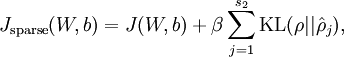
代價函式  為:
為:
![\begin{align}
J(W,b)
&= \left[ \frac{1}{m} \sum_{i=1}^m J(W,b;x^{(i)},y^{(i)}) \right]
+ \frac{\lambda}{2} \sum_{l=1}^{n_l-1} \; \sum_{i=1}^{s_l} \; \sum_{j=1}^{s_{l+1}} \left( W^{(l)}_{ji} \right)^2
\\
&= \left[ \frac{1}{m} \sum_{i=1}^m \left( \frac{1}{2} \left\| h_{W,b}(x^{(i)}) - y^{(i)} \right\|^2 \right) \right]
+ \frac{\lambda}{2} \sum_{l=1}^{n_l-1} \; \sum_{i=1}^{s_l} \; \sum_{j=1}^{s_{l+1}} \left( W^{(l)}_{ji} \right)^2
\end{align}](http://ufldl.stanford.edu/wiki/images/math/4/5/3/4539f5f00edca977011089b902670513.png)
 ,其中
,其中 ![\begin{align}
\hat\rho_j = \frac{1}{m} \sum_{i=1}^m \left[ a^{(2)}_j(x^{(i)}) \right]
\end{align}](http://ufldl.stanford.edu/wiki/images/math/8/7/2/8728009d101b17918c7ef40a6b1d34bb.png)
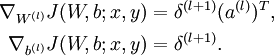
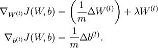
計算梯度需要用到的公式:
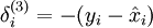 ,其中y是期望的輸出。
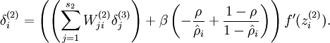 其中,
其中, 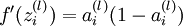
令  ,
, 


疑問
1.從程式碼中可看出,為什麼對10萬張小影象塊要經過預處理(0均值化和ZCA白化),而對2000張和3200張64*64RGB圖片卻未進行預處理?感覺自己對什麼時候該進行預處理,什麼時候不用進行預處理,為什麼這樣,都沒完全掌握!比如:在Deep Learning四之深度學習UFLDL教程:PCA in 2D_Exercise(斯坦福大學深度學習教程)中為什麼二維資料不用進行0均值化,而自然影象就要先0均值化?
實驗步驟
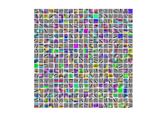
1.初始化引數,載入上一節實驗結果,即:10萬張8*8的RGB小影象塊中提取的顏色特徵,並把特徵視覺化。
2.先載入8張64*64的圖片(用來測試卷積和池化是否正確),再實現卷積函式cnnConvolve.m,並檢查該函式是否正確。
3.實現池化函式cnnPool.m,並檢查該函式是否正確。
4.載入2000張64*64RGB圖片,利用前面實現的卷積函式從中提取出卷積特徵convolvedFeaturesThis後,再利用池化函式從convolvedFeaturesThis中提取出池化特徵pooledFeaturesTrain,把它作為softmax分類器的訓練資料集;載入3200張64*64RGB圖片,利用前面實現的卷積函式從中提取出卷積特徵convolvedFeaturesThis後,再利用池化函式從convolvedFeaturesThis中提取出池化特徵pooledFeaturesTest,把它作為softmax分類器的測試資料集。
5.用訓練資料集pooledFeaturesTrain及其標籤訓練softmax分類器,得到模型引數softmaxModel。
6.利用訓練過的模型引數為pooledFeaturesTest的softmax分類器對測試資料集pooledFeaturesTest進行分類,即得到3200張64*64RGB圖片的分類結果。
執行結果
Accuracy: 80.313%
所有訓練資料和測試資料的卷積和池化特徵的提取所用時間為:
Elapsed time is 2644.920372 seconds.
特徵視覺化結果:
程式碼
cnnExercise.m
%% CS294A/CS294W Convolutional Neural Networks Exercise

%  Instructions
%  ------------
%
%  This file contains code that helps you get started on the
%  convolutional neural networks exercise. In this exercise, you will only
%  need to modify cnnConvolve.m and cnnPool.m. You will not need to modify
%  this file.

%%======================================================================
%% STEP 0: Initialization
%  Here we initialize some parameters used for the exercise.

imageDim = 64;         % image dimension
imageChannels = 3;     % number of channels (rgb, so 3)

patchDim = 8;          % patch dimension
numPatches = 50000;    % number of patches

visibleSize = patchDim * patchDim * imageChannels;  % number of input units
outputSize = visibleSize;   % number of output units
hiddenSize = 400;           % number of hidden units

epsilon = 0.1;           % epsilon for ZCA whitening

poolDim = 19;          % dimension of pooling region

%%======================================================================
%% STEP 1: Train a sparse autoencoder (with a linear decoder) to learn
%  features from color patches. If you have completed the linear decoder
%  execise, use the features that you have obtained from that exercise,
%  loading them into optTheta. Recall that we have to keep around the
%  parameters used in whitening (i.e., the ZCA whitening matrix and the
%  meanPatch)

% --------------------------- YOUR CODE HERE --------------------------
% Train the sparse autoencoder and fill the following variables with
% the optimal parameters:

optTheta =  zeros(2*hiddenSize*visibleSize+hiddenSize+visibleSize, 1);
ZCAWhite =  zeros(visibleSize, visibleSize);
meanPatch = zeros(visibleSize, 1);
load STL10Features.mat;

% --------------------------------------------------------------------

% Display and check to see that the features look good
W = reshape(optTheta(1:visibleSize * hiddenSize), hiddenSize, visibleSize);
b = optTheta(2*hiddenSize*visibleSize+1:2*hiddenSize*visibleSize+hiddenSize);

displayColorNetwork( (W*ZCAWhite)');

%%======================================================================
%% STEP 2: Implement and test convolution and pooling
%  In this step, you will implement convolution and pooling, and test them
%  on a small part of the data set to ensure that you have implemented
%  these two functions correctly. In the next step, you will actually
%  convolve and pool the features with the STL10 images.

%% STEP 2a: Implement convolution
%  Implement convolution in the function cnnConvolve in cnnConvolve.m

% Note that we have to preprocess the images in the exact same way
% we preprocessed the patches before we can obtain the feature activations.

load stlTrainSubset.mat % loads numTrainImages, trainImages, trainLabels

%% 只用8張圖片來測試卷積和池化是否正確 Use only the first 8 images for testing
convImages = trainImages(:, :, :, 1:8);  % 格式:trainImages(r, c, channel, image number)

% NOTE: Implement cnnConvolve in cnnConvolve.m first!
convolvedFeatures = cnnConvolve(patchDim, hiddenSize, convImages, W, b, ZCAWhite, meanPatch);

%% STEP 2b: Checking your convolution
%  To ensure that you have convolved the features correctly, we have
%  provided some code to compare the results of your convolution with
%  activations from the sparse autoencoder

% For 1000 random points
for i = 1:1000
    featureNum = randi([1, hiddenSize]);
    imageNum = randi([1, 8]);
    imageRow = randi([1, imageDim - patchDim + 1]);
    imageCol = randi([1, imageDim - patchDim + 1]);

    patch = convImages(imageRow:imageRow + patchDim - 1, imageCol:imageCol + patchDim - 1, :, imageNum);
    patch = patch(:);  % 將patch矩陣從3維矩陣轉換為一個列向量
    patch = patch - meanPatch;
    patch = ZCAWhite * patch;  % 白化後的資料

    features = feedForwardAutoencoder(optTheta, hiddenSize, visibleSize, patch);

    if abs(features(featureNum, 1) - convolvedFeatures(featureNum, imageNum, imageRow, imageCol)) > 1e-9
        fprintf('Convolved feature does not match activation from autoencoder\n');
        fprintf('Feature Number    : %d\n', featureNum);
        fprintf('Image Number      : %d\n', imageNum);
        fprintf('Image Row         : %d\n', imageRow);
        fprintf('Image Column      : %d\n', imageCol);
        fprintf('Convolved feature : %0.5f\n', convolvedFeatures(featureNum, imageNum, imageRow, imageCol));
        fprintf('Sparse AE feature : %0.5f\n', features(featureNum, 1));
        error('Convolved feature does not match activation from autoencoder');
    end
end

disp('Congratulations! Your convolution code passed the test.');

%% STEP 2c: Implement pooling
%  Implement pooling in the function cnnPool in cnnPool.m

% NOTE: Implement cnnPool in cnnPool.m first!
pooledFeatures = cnnPool(poolDim, convolvedFeatures);

%% STEP 2d: Checking your pooling
%  To ensure that you have implemented pooling, we will use your pooling
%  function to pool over a test matrix and check the results.

testMatrix = reshape(1:64, 8, 8);
expectedMatrix = [mean(mean(testMatrix(1:4, 1:4))) mean(mean(testMatrix(1:4, 5:8))); ...
                  mean(mean(testMatrix(5:8, 1:4))) mean(mean(testMatrix(5:8, 5:8))); ];

testMatrix = reshape(testMatrix, 1, 1, 8, 8);

pooledFeatures = squeeze(cnnPool(4, testMatrix));

if ~isequal(pooledFeatures, expectedMatrix)
    disp('Pooling incorrect');
    disp('Expected');
    disp(expectedMatrix);
    disp('Got');
    disp(pooledFeatures);
else
    disp('Congratulations! Your pooling code passed the test.');
end

%%======================================================================
%% STEP 3: Convolve and pool with the dataset
%  In this step, you will convolve each of the features you learned with
%  the full large images to obtain the convolved features. You will then
%  pool the convolved features to obtain the pooled features for
%  classification.
%
%  Because the convolved features matrix is very large, we will do the
%  convolution and pooling 50 features at a time to avoid running out of
%  memory. Reduce this number if necessary

stepSize = 50;
assert(mod(hiddenSize, stepSize) == 0, 'stepSize should divide hiddenSize');

load stlTrainSubset.mat % loads numTrainImages, trainImages, trainLabels
load stlTestSubset.mat  % loads numTestImages,  testImages,  testLabels

pooledFeaturesTrain = zeros(hiddenSize, numTrainImages, ...
    floor((imageDim - patchDim + 1) / poolDim), ...
    floor((imageDim - patchDim + 1) / poolDim) );
pooledFeaturesTest = zeros(hiddenSize, numTestImages, ...
    floor((imageDim - patchDim + 1) / poolDim), ...
    floor((imageDim - patchDim + 1) / poolDim) );

tic();

for convPart = 1:(hiddenSize / stepSize)

    featureStart = (convPart - 1) * stepSize + 1;
    featureEnd = convPart * stepSize;

    fprintf('Step %d: features %d to %d\n', convPart, featureStart, featureEnd);
    Wt = W(featureStart:featureEnd, :);
    bt = b(featureStart:featureEnd);

    fprintf('Convolving and pooling train images\n');
    convolvedFeaturesThis = cnnConvolve(patchDim, stepSize, ...
        trainImages, Wt, bt, ZCAWhite, meanPatch);
    pooledFeaturesThis = cnnPool(poolDim, convolvedFeaturesThis);
    pooledFeaturesTrain(featureStart:featureEnd, :, :, :) = pooledFeaturesThis;
    toc();
    clear convolvedFeaturesThis pooledFeaturesThis;

    fprintf('Convolving and pooling test images\n');
    convolvedFeaturesThis = cnnConvolve(patchDim, stepSize, ...
        testImages, Wt, bt, ZCAWhite, meanPatch);
    pooledFeaturesThis = cnnPool(poolDim, convolvedFeaturesThis);
    pooledFeaturesTest(featureStart:featureEnd, :, :, :) = pooledFeaturesThis;
    toc();

    clear convolvedFeaturesThis pooledFeaturesThis;

end


% You might want to save the pooled features since convolution and pooling takes a long time
save('cnnPooledFeatures.mat', 'pooledFeaturesTrain', 'pooledFeaturesTest');
toc();

%%======================================================================
%% STEP 4: Use pooled features for classification
%  Now, you will use your pooled features to train a softmax classifier,
%  using softmaxTrain from the softmax exercise.
%  Training the softmax classifer for 1000 iterations should take less than
%  10 minutes.

% Add the path to your softmax solution, if necessary
% addpath /path/to/solution/

% Setup parameters for softmax
softmaxLambda = 1e-4;
numClasses = 4;
% Reshape the pooledFeatures to form an input vector for softmax
softmaxX = permute(pooledFeaturesTrain, [1 3 4 2]); % 把pooledFeaturesTrain的第2維移到最後
softmaxX = reshape(softmaxX, numel(pooledFeaturesTrain) / numTrainImages,...
    numTrainImages);
softmaxY = trainLabels;

options = struct;
options.maxIter = 200;
softmaxModel = softmaxTrain(numel(pooledFeaturesTrain) / numTrainImages,...
    numClasses, softmaxLambda, softmaxX, softmaxY, options);

%%======================================================================
%% STEP 5: Test classifer
%  Now you will test your trained classifer against the test images

softmaxX = permute(pooledFeaturesTest, [1 3 4 2]);
softmaxX = reshape(softmaxX, numel(pooledFeaturesTest) / numTestImages, numTestImages);
softmaxY = testLabels;

[pred] = softmaxPredict(softmaxModel, softmaxX);
acc = (pred(:) == softmaxY(:));
acc = sum(acc) / size(acc, 1);
fprintf('Accuracy: %2.3f%%\n', acc * 100);

% You should expect to get an accuracy of around 80% on the test images.
cnnConvolve.m
function convolvedFeatures = cnnConvolve(patchDim, numFeatures, images, W, b, ZCAWhite, meanPatch)
%卷積特徵提取:把每一個特徵都與每一張大尺寸圖片images相卷積,並返回卷積結果
%cnnConvolve Returns the convolution of the features given by W and b with
%the given images
%
% Parameters:
%  patchDim - patch (feature) dimension
%  numFeatures - number of features
%  images - large images to convolve with, matrix in the form
%           images(r, c, channel, image number)
%  W, b - W, b for features from the sparse autoencoder
%  ZCAWhite, meanPatch - ZCAWhitening and meanPatch matrices used for
%                        preprocessing
%
% Returns:
%  convolvedFeatures - matrix of convolved features in the form
%                      convolvedFeatures(featureNum, imageNum, imageRow, imageCol)
%                      表示第個featureNum特徵與第imageNum張圖片相卷的結果儲存在矩陣
%                      convolvedFeatures(featureNum, imageNum, :, :)的第imageRow行第imageCol列,
%                      而每行和列的大小都為imageDim - patchDim + 1

numImages = size(images, 4);     % 圖片數量
imageDim = size(images, 1);      % 每幅圖片行數
imageChannels = size(images, 3); % 每幅圖片通道數

patchSize = patchDim*patchDim;
assert(numFeatures == size(W,1), 'W should have numFeatures rows');
assert(patchSize*imageChannels == size(W,2), 'W should have patchSize*imageChannels cols');


% Instructions:
%   Convolve every feature with every large image here to produce the
%   numFeatures x numImages x (imageDim - patchDim + 1) x (imageDim - patchDim + 1)
%   matrix convolvedFeatures, such that
%   convolvedFeatures(featureNum, imageNum, imageRow, imageCol) is the
%   value of the convolved featureNum feature for the imageNum image over
%   the region (imageRow, imageCol) to (imageRow + patchDim - 1, imageCol + patchDim - 1)
%
% Expected running times:
%   Convolving with 100 images should take less than 3 minutes
%   Convolving with 5000 images should take around an hour
%   (So to save time when testing, you should convolve with less images, as
%   described earlier)

% -------------------- YOUR CODE HERE --------------------
% Precompute the matrices that will be used during the convolution. Recall
% that you need to take into account the whitening and mean subtraction
% steps

WT = W*ZCAWhite;           % 等效的網路權值
b_mean = b - WT*meanPatch; % 等效偏置項


% --------------------------------------------------------

convolvedFeatures = zeros(numFeatures, numImages, imageDim - patchDim + 1, imageDim - patchDim + 1);
for imageNum = 1:numImages
  for featureNum = 1:numFeatures

    % convolution of image with feature matrix for each channel
    convolvedImage = zeros(imageDim - patchDim + 1, imageDim - patchDim + 1);
    for channel = 1:3

      % Obtain the feature (patchDim x patchDim) needed during the convolution
      % ---- YOUR CODE HERE ----
      offset = (channel-1)*patchSize;
      feature = reshape(WT(featureNum,offset+1:offset+patchSize), patchDim, patchDim);%取一個權值影象塊出來
      im  = images(:,:,channel,imageNum);


      % ------------------------

      % Flip the feature matrix because of the definition of convolution, as explained later
      feature = rot90(squeeze(feature),2);

      % Obtain the image
      im = squeeze(images(:, :, channel, imageNum));

      % Convolve "feature" with "im", adding the result to convolvedImage
      % be sure to do a 'valid' convolution
      % ---- YOUR CODE HERE ----

      convolvedoneChannel = conv2(im, feature, 'valid');    % 單個特徵分別與所有圖片相卷
      convolvedImage = convolvedImage + convolvedoneChannel;% 直接把3通道的值加起來,理由:3通道相當於有3個feature-map,類似於cnn第2層以後的輸入。

      % ------------------------

    end

    % Subtract the bias unit (correcting for the mean subtraction as well)
    % Then, apply the sigmoid function to get the hidden activation
    % ---- YOUR CODE HERE ----

    convolvedImage = sigmoid(convolvedImage+b_mean(featureNum));


    % ------------------------

    % The convolved feature is the sum of the convolved values for all channels
    convolvedFeatures(featureNum, imageNum, :, :) = convolvedImage;
  end
end


end
function sigm = sigmoid(x)
    sigm = 1./(1+exp(-x));
end
cnnPool.m
function pooledFeatures = cnnPool(poolDim, convolvedFeatures)
%cnnPool Pools the given convolved features
%
% Parameters:
%  poolDim - dimension of pooling region
%  convolvedFeatures - convolved features to pool (as given by cnnConvolve)
%                      convolvedFeatures(featureNum, imageNum, imageRow, imageCol)
%
% Returns:
%  pooledFeatures - matrix of pooled features in the form
%                   pooledFeatures(featureNum, imageNum, poolRow, poolCol)
%                      表示第個featureNum特徵與第imageNum張圖片的卷積特徵池化後的結果儲存在矩陣
%                      pooledFeatures(featureNum, imageNum, :, :)的第poolRow行第poolCol列
%

numImages = size(convolvedFeatures, 2);   % 圖片數量
numFeatures = size(convolvedFeatures, 1); % 卷積特徵數量
convolvedDim = size(convolvedFeatures, 3);% 卷積特徵維數

pooledFeatures = zeros(numFeatures, numImages, floor(convolvedDim / poolDim), floor(convolvedDim / poolDim));

% -------------------- YOUR CODE HERE --------------------
% Instructions:
%   Now pool the convolved features in regions of poolDim x poolDim,
%   to obtain the
%   numFeatures x numImages x (convolvedDim/poolDim) x (convolvedDim/poolDim)
%   matrix pooledFeatures, such that
%   pooledFeatures(featureNum, imageNum, poolRow, poolCol) is the
%   value of the featureNum feature for the imageNum image pooled over the
%   corresponding (poolRow, poolCol) pooling region
%   (see http://ufldl/wiki/index.php/Pooling )
%
%   Use mean pooling here.
% -------------------- YOUR CODE HERE --------------------

resultDim  = floor(convolvedDim / poolDim);
for imageNum = 1:numImages   % 第imageNum張圖片
    for featureNum = 1:numFeatures  % 第featureNum個特徵
        for poolRow = 1:resultDim
            offsetRow = 1+(poolRow-1)*poolDim;
            for poolCol = 1:resultDim
                offsetCol = 1+(poolCol-1)*poolDim;
                patch = convolvedFeatures(featureNum,imageNum,offsetRow:offsetRow+poolDim-1,...
                    offsetCol:offsetCol+poolDim-1);%取出一個patch
                pooledFeatures(featureNum,imageNum,poolRow,poolCol) = mean(patch(:));%使用均值pool
            end
        end
    end
end


end
參考資料
——
相關推薦
Deep Learning 10_深度學習UFLDL教程:Convolution and Pooling_exercise(斯坦福大學深度學習教程)
前言 實驗環境:win7, matlab2015b,16G記憶體,2T機械硬碟 實驗內容:Exercise:Convolution and Pooling。從2000張64*64的RGB圖片(它是 the STL10 Dataset的一個子集)中提取特徵作為訓練資料集,訓練softmax分類器,然後從
Deep Learning 5_深度學習UFLDL教程:PCA and Whitening_Exercise(斯坦福大學深度學習教程)
close all; % clear all; %%================================================================ %% Step 0a: Load data % Here we provide the code to load n
Deep Learning 1_深度學習UFLDL教程:Sparse Autoencoder練習(斯坦福大學深度學習教程)
1前言 本人寫技術部落格的目的,其實是感覺好多東西,很長一段時間不動就會忘記了,為了加深學習記憶以及方便以後可能忘記後能很快回憶起自己曾經學過的東西。 首先,在網上找了一些資料,看見介紹說UFLDL很不錯,很適合從基礎開始學習,Adrew Ng大牛寫得一點都不裝B,感覺非常好
Deep Learning 4_深度學習UFLDL教程:PCA in 2D_Exercise(斯坦福大學深度學習教程)
前言 本節練習的主要內容:PCA,PCA Whitening以及ZCA Whitening在2D資料上的使用,2D的資料集是45個數據點,每個資料點是2維的。要注意區別比較二維資料與二維影象的不同,特別是在程式碼中,可以看出主要二維資料的在PCA前的預處理不需要先0均值歸一化,而二維自然影象需要先
Deep Learning 19_深度學習UFLDL教程:Convolutional Neural Network_Exercise(斯坦福大學深度學習教程)
基礎知識 概述 CNN是由一個或多個卷積層(其後常跟一個下采樣層)和一個或多個全連線層組成的多層神經網路。CNN的輸入是2維影象(或者其他2維輸入,如語音訊號)。它通過區域性連線和權值共享,再通過池化可得到平移不變特徵。CNN的另一個優點就是易於訓練
Deep Learning 11_深度學習UFLDL教程:資料預處理(斯坦福大學深度學習教程)
資料預處理是深度學習中非常重要的一步!如果說原始資料的獲得,是深度學習中最重要的一步,那麼獲得原始資料之後對它的預處理更是重要的一部分。 1.資料預處理的方法: ①資料歸一化: 簡單縮放:對資料的每一個維度的值進行重新調節,使其在 [0,1]或[ − 1,1] 的區間內 逐樣本均值消減:在每個
Deep Learning 13_深度學習UFLDL教程:Independent Component Analysis_Exercise(斯坦福大學深度學習教程)
前言 實驗環境:win7, matlab2015b,16G記憶體,2T機械硬碟 難點:本實驗難點在於執行時間比較長,跑一次都快一天了,並且我還要驗證各種代價函式的對錯,所以跑了很多次。 實驗基礎說明: ①不同點:本節實驗中的基是標準正交的,也是線性獨立的,而Deep Learni
Deep Learning 7_深度學習UFLDL教程:Self-Taught Learning_Exercise(斯坦福大學深度學習教程)
前言 理論知識:自我學習 練習環境:win7, matlab2015b,16G記憶體,2T硬碟 一是用29404個無標註資料unlabeledData(手寫數字資料庫MNIST Dataset中數字為5-9的資料)來訓練稀疏自動編碼器,得到其權重引數opttheta。這一步的目的是提取這
Deep Learning 2_深度學習UFLDL教程:向量化程式設計(斯坦福大學深度學習教程)
1前言 本節主要是讓人用向量化程式設計代替效率比較低的for迴圈。 在前一節的Sparse Autoencoder練習中已經實現了向量化程式設計,所以與前一節的區別只在於本節訓練集是用MINIST資料集,而上一節訓練集用的是從10張圖片中隨機選擇的8*8的10000張小圖塊。綜上,只需要在
Deep Learning 3_深度學習UFLDL教程:預處理之主成分分析與白化_總結(斯坦福大學深度學習教程)
1PCA ①PCA的作用:一是降維;二是可用於資料視覺化; 注意:降維的原因是因為原始資料太大,希望提高訓練速度但又不希望產生很大的誤差。 ② PCA的使用場合:一是希望提高訓練速度;二是記憶體太小;三是希望資料視覺化。 ③用PCA前的預處理:(1)規整化特徵的均值大致為0;(
Deep Learning 8_深度學習UFLDL教程:Stacked Autocoders and Implement deep networks for digit classification_Exercise(斯坦福大學深度學習教程)
前言 2.實驗環境:win7, matlab2015b,16G記憶體,2T硬碟 3.實驗內容:Exercise: Implement deep networks for digit classification。利用深度網路完成MNIST手寫數字資料庫中手寫數字的識別。即:用6萬個已標註資料(即:6萬
Deep Learning 12_深度學習UFLDL教程:Sparse Coding_exercise(斯坦福大學深度學習教程)
前言 實驗環境:win7, matlab2015b,16G記憶體,2T機械硬碟 本節實驗比較不好理解也不好做,我看很多人最後也沒得出好的結果,所以得花時間仔細理解才行。 實驗內容:Exercise:Sparse Coding。從10張512*512的已經白化後的灰度影象(即:Deep Learnin
Deep Learning 6_深度學習UFLDL教程:Softmax Regression_Exercise(斯坦福大學深度學習教程)
前言 練習內容:Exercise:Softmax Regression。完成MNIST手寫數字資料庫中手寫數字的識別,即:用6萬個已標註資料(即:6萬張28*28的影象塊(patches)),作訓練資料集,然後利用其訓練softmax分類器,再用1萬個已標註資料(即:1萬張28*28的影象塊(pa
Deep Learning 9_深度學習UFLDL教程:linear decoder_exercise(斯坦福大學深度學習教程)
前言 實驗基礎說明: 1.為什麼要用線性解碼器,而不用前面用過的棧式自編碼器等?即:線性解碼器的作用? 這一點,Ng已經在講解中說明了,因為線性解碼器不用要求輸入資料範圍一定為(0,1),而前面用過的棧式自編碼器等要求輸入資料範圍必須為(0,1)。因為a3的輸出值是f函式的輸出,而在普通的spa
實時翻譯的發動機:矢量語義(斯坦福大學課程解讀)
處理 多個 abi rod 進一步 ews 有一種 deb rac
CodeForces - 367E:Sereja and Intervals(組合數&&DP)
ant lov strong clas require sequence 組合 pri c++ Sereja is interested in intervals of numbers, so he has prepared a problem about interval
Keras TensorFlow教程:如何從零開發一個複雜深度學習模型
Keras 是提供一些高可用的 Python API ,能幫助你快速的構建和訓練自己的深度學習模型,它的後端是 TensorFlow 或者 Theano 。本文假設你已經熟悉了 TensorFlow 和卷積神經網路,如果,你還沒有熟悉,那麼可以先看看這個10分鐘入門 TensorFlow 教程和卷積
斯坦福大學公開課機器學習:advice for applying machine learning | learning curves (改進學習算法:高偏差和高方差與學習曲線的關系)
繪制 學習曲線 pos 情況 但我 容量 繼續 並且 inf 繪制學習曲線非常有用,比如你想檢查你的學習算法,運行是否正常。或者你希望改進算法的表現或效果。那麽學習曲線就是一種很好的工具。學習曲線可以判斷某一個學習算法,是偏差、方差問題,或是二者皆有。 為了繪制一條學習曲
CS294-112深度增強學習課程(加州大學伯克利分校 2017)NO.3 Learning dynamical system models from data
增強 data learning http src img sys 增強學習 學習
《TensorFlow:實戰Google深度學習框架》——5.4 模型持久化(模型儲存、模型載入)
目錄 1、持久化程式碼實現 2、載入儲存的TensorFlow模型 3、載入部分變數 4、載入變數時重新命名 1、持久化程式碼實現 TensorFlow提供了一個非常簡單的API來儲存和還原一個神經網路模型。這個API就是tf.train.Saver類。一下程式碼給出了儲