這篇文章主要介紹一個有效的資料降維的方法 t-SNE.

大資料時代，資料量不僅急劇膨脹，資料也變得越來越複雜，資料的維度也隨之增加。比如大圖片，資料維度指的是畫素的數量級，範圍從數千到數百萬。計算機可以處理任意多維的資料集，但我們人類認知只侷限於3維空間，計算機依然需要我們（值得慶幸的），所以需要通過一些方法有效的視覺化高維資料。通過觀察現實世界的資料集發現其存在一些較低的本徵維度。想像一下你拿著相機在拍照，可以把每張圖片認為是16，000，000維空間的點（假設相機是16畫素的），但是這些照片是近似分佈在三維空間，這個低維空間使用一個複雜的、非線性的方法嵌入到高維空間，這種結構隱藏在資料中，只有通過一定的數學分析方法還原。
這裡講到的是流行學習方法，也可以說非線性降維方法，ML的一個分支（更具體的說，是非監督學習）。這篇文章主要講到一個流行的資料降維的方法t-SNE，由Laurens vander Maaten和 Geoffrey Hinton提出（

視覺化mnist
首先import一些libraries。

import numpy as np
from numpy import linalg
from numpy.linalg import norm
from scipy.spatial.distance import squareform, pdist

再import sklearn

import sklearn
from sklearn.manifold import TSNE
from
 
 sklearn.datasets import load_digits
from sklearn.preprocessing import scale
from sklearn.metrics.pairwise import pairwise_distances
from sklearn.manifold.t_sne import (_joint_probabilities,
                                    _kl_divergence)
from sklearn.utils.extmath import _ravel

隨機狀態值

RS = 20150101
 

使用圖形庫matplotlib

import matplotlib.pyplot as plt
import matplotlib.patheffects as PathEffects
import matplotlib
%matplotlib inline

使用seaborn更好繪製圖

import seaborn as sns
sns.set_style('darkgrid')
sns.set_palette('muted')
sns.set_context("notebook", font_scale=1.5,
                rc={"lines.linewidth": 2.5})

使用matplotlib 和 moviepy生成動畫

from moviepy.video.io.bindings import mplfig_to_npimage
import moviepy.editor as mpy

載入手寫數字識別庫，共有1797張圖片，每張大小8X8

digits = load_digits()
digits.data.shape
print(digits['DESCR'])

Data Set Characteristics:
:Number of Instances: 5620
:Number of Attributes: 64
:Attribute Information: 8x8 image of integer pixels in the range 0..16.
:Missing Attribute Values: None

nrows, ncols = 2, 5
plt.figure(figsize=(6,3))
plt.gray()
for i in range(ncols * nrows):
    ax = plt.subplot(nrows, ncols, i + 1)
    ax.matshow(digits.images[i,...])
    plt.xticks([]); plt.yticks([])
    plt.title(digits.target[i])
plt.savefig('images/digits-generated.png', dpi=150)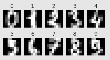

現在執行t-SNE演算法：

X = np.vstack([digits.data[digits.target==i]
               for i in range(10)])
y = np.hstack([digits.target[digits.target==i]
               for i in range(10)])
digits_proj = TSNE(random_state=RS).fit_transform(X)              

下面是一個顯示轉換後資料集的函式

def scatter(x, colors):
    # We choose a color palette with seaborn.
    palette = np.array(sns.color_palette("hls", 10))

    # We create a scatter plot.
    f = plt.figure(figsize=(8, 8))
    ax = plt.subplot(aspect='equal')
    sc = ax.scatter(x[:,0], x[:,1], lw=0, s=40,
                    c=palette[colors.astype(np.int)])
    plt.xlim(-25, 25)
    plt.ylim(-25, 25)
    ax.axis('off')
    ax.axis('tight')

    # We add the labels for each digit.
    txts = []
    for i in range(10):
        # Position of each label.
        xtext, ytext = np.median(x[colors == i, :], axis=0)
        txt = ax.text(xtext, ytext, str(i), fontsize=24)
        txt.set_path_effects([
            PathEffects.Stroke(linewidth=5, foreground="w"),
            PathEffects.Normal()])
        txts.append(txt)

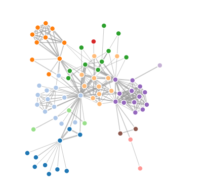
    return f, ax, sc, txts

結果：

scatter(digits_proj, y)
plt.savefig('images/digits_tsne-generated.png', dpi=120)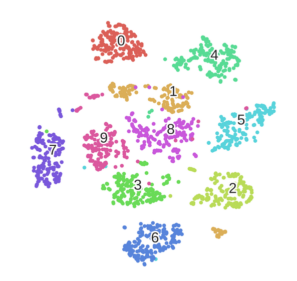

不同顏色的點代表不同的數字，可以觀察到相同的數字被清晰的分到不同的聚集區域.

數學框架
下面介紹演算法的工作原理。首先，介紹幾個定義：
資料點X_i分佈在原始資料空間R^D,資料空間的維度為D=64，每個點代表手寫數字識別庫中的每張圖片。總共有N=1797個點。
對映點y_i在對映空間R^2，對映空間是我們對資料的最終表達。資料點和對映點之間存在雙射關係，一個對映點表示一張原始圖片。
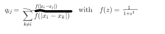
我們該怎樣選擇對映點的位置呢？如果兩個資料點距離比較近，我們希望對應的兩個對映點的位置也相對比較接近。另|x_i−x_j|計算兩個資料點間的歐式距離，|y_i−y_j| 表示對映點的距離。首先定義兩資料點間的條件相似性：

公式度量了x_i與x_j的距離，σ_i^2為滿足高斯分佈的x_i的方差。原文詳細講解方差的計算，這裡不再寫。
現在定義相似度：

我們從原始影象獲得一個相似矩陣，這個矩陣是怎樣的呢？
相似矩陣
下面的函式定義了計算相似矩陣函式，常量 σ：

def _joint_probabilities_constant_sigma(D, sigma):
    P = np.exp(-D**2/2 * sigma**2)
    P /= np.sum(P, axis=1)
    return P

# Pairwise distances between all data points.
D = pairwise_distances(X, squared=True)
# Similarity with constant sigma.
P_constant = _joint_probabilities_constant_sigma(D, .002)
# Similarity with variable sigma.
P_binary = _joint_probabilities(D, 30., False)
# The output of this function needs to be reshaped to a square matrix.
P_binary_s = squareform(P_binary)

現在可以顯示資料點的距離陣：

plt.figure(figsize=(12, 4))
pal = sns.light_palette("blue", as_cmap=True)

plt.subplot(131)
plt.imshow(D[::10, ::10], interpolation='none', cmap=pal)
plt.axis('off')
plt.title("Distance matrix", fontdict={'fontsize': 16})

plt.subplot(132)
plt.imshow(P_constant[::10, ::10], interpolation='none', cmap=pal)
plt.axis('off')
plt.title("$p_{j|i}$ (constant $\sigma$)", fontdict={'fontsize': 16})

plt.subplot(133)
plt.imshow(P_binary_s[::10, ::10], interpolation='none', cmap=pal)
plt.axis('off')
plt.title("$p_{j|i}$ (variable $\sigma$)", fontdict={'fontsize': 16})
plt.savefig('images/similarity-generated.png', dpi=120)

接下來定義對映點的相似矩陣：

pij和qij足夠的接近，即達到使資料點和對映點足夠接近的目的。

結構分析

如果兩個對映點距離較遠但是資料點較近，他們會相互吸引，當兩個對映點較遠資料點較近，他們會排斥。當達到平衡時獲得最後的對映。下面的插圖展示了這一特點：

演算法
以上物理的類比來源於數學的演算法，最小化兩個分佈的 Kullback-Leiber發散程度：

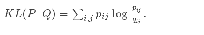
這裡度量了兩個相似矩陣的距離。
使用梯度下降最優化結果：

u_ij對應於y_j到y_i的向量，梯度表達的是作用在對映節點i上的所有彈縮力的和。

# This list will contain the positions of the map points at every iteration.
positions = []
def _gradient_descent(objective, p0, it, n_iter, n_iter_without_progress=30,
                      momentum=0.5, learning_rate=1000.0, min_gain=0.01,
                      min_grad_norm=1e-7, min_error_diff=1e-7, verbose=0,
                      args=[]):
    # The documentation of this function can be found in scikit-learn's code.
    p = p0.copy().ravel()
    update = np.zeros_like(p)
    gains = np.ones_like(p)
    error = np.finfo(np.float).max
    best_error = np.finfo(np.float).max
    best_iter = 0

    for i in range(it, n_iter):
        # We save the current position.
        positions.append(p.copy())

        new_error, grad = objective(p, *args)
        error_diff = np.abs(new_error - error)
        error = new_error
        grad_norm = linalg.norm(grad)

        if error < best_error:
            best_error = error
            best_iter = i
        elif i - best_iter > n_iter_without_progress:
            break
        if min_grad_norm >= grad_norm:
            break
        if min_error_diff >= error_diff:
            break

        inc = update * grad >= 0.0
        dec = np.invert(inc)
        gains[inc] += 0.05
        gains[dec] *= 0.95
        np.clip(gains, min_gain, np.inf)
        grad *= gains
        update = momentum * update - learning_rate * grad
        p += update

    return p, error, i
sklearn.manifold.t_sne._gradient_descent = _gradient_descent