
CS231n課程學習筆記(一)——KNN的實現
作業講解
KNN的實現主要分為兩步:
- 訓練:分類器簡單地記住所有的資料
- 測試:測試資料分別和所有訓練資料計算距離,選取k個最近的訓練樣本的label,通過投票(vote)獲得預測值。
在cs231n\classifiers資料夾中的 k_nearest_neighbor.py 完成KNN的實現程式碼
雙迴圈
每個測試資料和每個訓練資料分別計算(兩層迴圈),可以直接使用numpy中一個函式:np.linalg.norm()
for i in range(num_test):#測試樣本的迴圈
for j in range(num_train):#訓練樣本的迴圈 單迴圈
每個測試資料和訓練資料分別整體進行計算(一層迴圈),使用np.linalg.norm(),注意引數axis的設定(由於我們是在第一維求距離,因此axis=1)。
這裡其實使用了廣播機制broadcast,
X[i,:]維度為1×D,X_train[i,:]維度為 num_train×D,由於廣播機制,X[i,:]會被補為 num_train×D,再使其與X_train[i,:]進行運算,最終dist[i,:]維度為1×num_train。
程式碼如下:
for i in range(num_test):
#dists[i,:] = np.sqrt(np.sum(np.square(self.X_train-X[i,:]),axis = 1))
dists[i,:]=np.linalg.norm(X[i,:]-self.X_train[:],axis=1)無迴圈
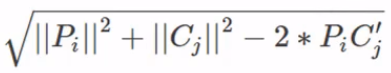
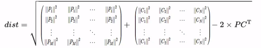
- 令測試集為,訓練集為,為測試資料資料量,為訓練資料資料量,是維度。實際上最後距離公式變為如下形式,注意 是矩陣乘(
np.dot())。這裡實現的依然是廣播,所以只要的形狀為 ,的形狀為 即可。
- 廣播:
具體實現程式碼如下:
"""
mul1 = np.multiply(np.dot(X,self.X_train.T),-2)
sq1 = np.sum(np.square(X),axis=1,keepdims = True)
sq2 = np.sum(np.square(self.X_train),axis=1)
dists = mul1+sq1+sq2
dists = np.sqrt(dists)
"""
dists += np.sum(np.multiply(X,X),axis=1,keepdims = True).reshape(num_test,1)
dists += np.sum(np.multiply(self.X_train,self.X_train),axis=1,keepdims = True).reshape(1,num_train)
dists += -2*np.dot(X,self.X_train.T)
dists = np.sqrt(dists) 預測
np.argsort() 可以對dists 進行排序選出k個最近的訓練樣本的下標
np.bincount() 會統計輸入陣列出現的頻數,返回的也是下標,結合np.argmax()就可以實現vote機制。
for i in range(num_test):
closest_y = []
closest_y = self.y_train[np.argsort(dists[i, :])[:k]].flatten()
c = Counter(closest_y)
y_pred[i]=c.most_common(1)[0][0]
"""
closest_y=self.y_train[np.argsort(dists[i, :])[:k]]
y_pred[i] = np.argmax(np.bincount(closest_y))
"""由於我使用np.bincount()時會報錯 object too deep for desired array,因此改為上面的程式碼。(錯誤原因還未找到……)
Nearest Neighbor 分類器的優劣
該分類器在訓練階段不需要花時間,然而在測試階段卻要花費大量時間,因為要將每一個測試圖片與所有訓練圖片比對。所以幾乎沒人用這個演算法
L1,L2 範數來進行畫素比較是不夠的,影象更多的是按背景和顏色被分類,而不是語義主體分身
如果想要使K-NN演算法實用,可以對資料特徵進行normalize,讓其均值為0,和單位方差。或者用PCA降維
總體程式碼展示
由於原始碼是python2環境下編譯的,而我的編譯環境是python3,難免會出現報錯,只要將python3的用法替換過去就行了。
開啟knn.ipynb
import random
import numpy as np
from cs231n.data_utils import load_CIFAR10
import matplotlib.pyplot as plt
plt.rcParams['figure.figsize'] = (10.0, 8.0) # set default size of plots
plt.rcParams['image.interpolation'] = 'nearest'
plt.rcParams['image.cmap'] = 'gray'
將 data_utils.py 中 import cPickle as pickle 改為 import pickle as pickle
讀取資料
# Load the raw CIFAR-10 data.
cifar10_dir = 'cs231n/datasets/cifar-10-batches-py'
X_train, y_train, X_test, y_test = load_CIFAR10(cifar10_dir)
# As a sanity check, we print out the size of the training and test data.
print ('Training data shape: ', X_train.shape)
print ('Training labels shape: ', y_train.shape)
print ('Test data shape: ', X_test.shape)
print ('Test labels shape: ', y_test.shape)- Error:’ascii’ codec can’t decode byte 0x8b in position 6
將 data_utils.py 中datadict = pickle.load(f)改為datadict = pickle.load(f,encoding='iso-8859-1')
OUTPUT:
Training data shape: (50000, 32, 32, 3)
Training labels shape: (50000,)
Test data shape: (10000, 32, 32, 3)
Test labels shape: (10000,)
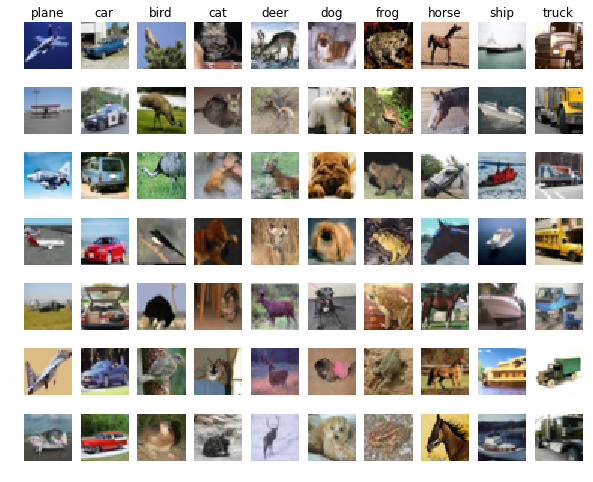
顯示樣本
# Visualize some examples from the dataset.
# We show a few examples of training images from each class.
classes = ['plane', 'car', 'bird', 'cat', 'deer', 'dog', 'frog', 'horse', 'ship', 'truck']
num_classes = len(classes)
samples_per_class = 7
for y, cls in enumerate(classes):
idxs = np.flatnonzero(y_train == y)
idxs = np.random.choice(idxs, samples_per_class, replace=False)
for i, idx in enumerate(idxs):
plt_idx = i * num_classes + y + 1
plt.subplot(samples_per_class, num_classes, plt_idx)
plt.imshow(X_train[idx].astype('uint8'))
plt.axis('off')
if i == 0:
plt.title(cls)
plt.show()OUTPUT:
numpy.flatnonzero():
該函式輸入一個矩陣,返回扁平化後矩陣中非零元素的位置(index)
enumerate()
返回一個可迭代物件的列舉形式,(上面第一個 返回 0 plane/ 1 car/ 2 bird/……)
調整資料集大小
# Subsample the data for more efficient code execution in this exercise
num_training = 5000
mask = range(num_training)
X_train = X_train[mask]
y_train = y_train[mask]
num_test = 500
mask = range(num_test)
X_test = X_test[mask]
y_test = y_test[mask]
# 把一張圖片變為一行向量
X_train = np.reshape(X_train, (X_train.shape[0], -1))
X_test = np.reshape(X_test, (X_test.shape[0], -1))
print(X_train.shape, X_test.shape)OUTPUT:(5000, 3072) (500, 3072)
KNN模型實現
在cs231n\classifiers資料夾中的 k_nearest_neighbor.py 完成KNN的實現程式碼。
由於每一個圖片用一行資料來表示,要得到測試圖片 j 與訓練圖片 i 的L2距離:
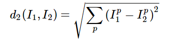
只需要將測試資料矩陣第 j 行的每一個點與訓練資料矩陣 第 i 行的每一個點平方求和再開方:
dist[i,j]=np.sqrt(np.sum(np.square(self.X_train[j,:]-X_test[i,:])))具體如下:
import numpy as np
from collections import Counter
class KNearestNeighbor(object):
""" a kNN classifier with L2 distance """
def __init__(self):
pass
def train(self, X, y):
self.X_train = X
self.y_train = y
def predict(self, X, k=1, num_loops=0):
if num_loops == 0:
dists = self.compute_distances_no_loops(X)
elif num_loops == 1:
dists = self.compute_distances_one_loop(X)
elif num_loops == 2:
dists = self.compute_distances_two_loops(X)
else:
raise ValueError('Invalid value %d for num_loops' % num_loops)
return self.predict_labels(dists, k=k)
def compute_distances_two_loops(self, X):
num_test = X.shape[0]
num_train = self.X_train.shape[0]
dists = np.zeros((num_test, num_train))
for i in range(num_test):#測試樣本的迴圈
  for j in range(num_train):#訓練樣本的迴圈
    #dists[i,j]=np.sqrt(np.sum(np.square(self.X_train[j,:]-X[i,:])))
    dists[i,j]=np.linalg.norm(X[i]-self.X_train[j])
#np.square是針對每個元素的平方方法
return dists
def compute_distances_one_loop(self, X):
num_test = X.shape[0]
num_train = self.X_train.shape[0]
dists = np.zeros((num_test, num_train))
for i in range(num_test):
   #dists[i,:] = np.sqrt(np.sum(np.square(self.X_train-X[i,:]),axis = 1))
   dists[i,:]=np.linalg.norm(X[i,:]-self.X_train[:],axis=1)
return dists
def compute_distances_no_loops(self, X):
num_test = X.shape[0]
num_train = self.X_train.shape[0]
dists = np.zeros((num_test, num_train))
"""
mul1 = np.multiply(np.dot(X,self.X_train.T),-2)
sq1 = np.sum(np.square(X),axis=1,keepdims = True)
sq2 = np.sum(np.square(self.X_train),axis=1)
dists = mul1+sq1+sq2
dists = np.sqrt(dists)
"""
dists += np.sum(np.multiply(X,X),axis=1,keepdims = True).reshape(num_test,1)
dists += np.sum(np.multiply(self.X_train,self.X_train),axis=1,keepdims = True).reshape(1,num_train)
dists += -2*np.dot(X,self.X_train.T)
dists = np.sqrt(dists)
return dists
def predict_labels(self, dists, k=1):
num_test = dists.shape[0]
y_pred = np.zeros(num_test)
for i in range(num_test):
  closest_y = []
  closest_y = self.y_train[np.argsort(dists[i, :])[:k]].flatten()
  c = Counter(closest_y)
  y_pred[i]=c.most_common(1)[0][0]
  """
  closest_y=self.y_train[np.argsort(dists[i, :])[:k]]
  y_pred[i] = np.argmax(np.bincount(closest_y))
  """
return y_prednumpy.bincount詳見這裡
訓練模型
knn.ipynb:匯入KNN模型
from cs231n.classifiers import KNearestNeighbor

classifier = KNearestNeighbor()
classifier.train(X_train, y_train)

dists = classifier.compute_distances_two_loops(X_test)
print (dists.shape) #>> (500,5000)

y_test_pred = classifier.predict_labels(dists, k=1)

#計算兩層迴圈的結果
num_correct = np.sum(y_test_pred == y_test)
accuracy = float(num_correct) / num_test
print ('Got %d / %d correct => accuracy: %f' % (num_correct, num_test, accuracy))
#>>Got 137 / 500 correct => accuracy: 0.274000
#計算一層迴圈的結果
y_test_pred = classifier.predict_labels(dists, k=5)
num_correct = np.sum(y_test_pred == y_test)
accuracy = float(num_correct) / num_test
print ('Got %d / %d correct => accuracy: %f' % (num_correct, num_test, accuracy))
#>>Got 139 / 500 correct => accuracy: 0.278000

dists_one = classifier.compute_distances_one_loop(X_test)
#檢查兩次距離是否一樣 dists,dists_one
difference = np.linalg.norm(dists - dists_one, ord='fro')
print ('Difference was: %f' % (difference, ))
if difference < 0.001:
  print ('Good! The distance matrices are the same')
else:
  print ('Uh-oh! The distance matrices are different')

dists_two = classifier.compute_distances_no_loops(X_test)

#檢查兩次距離是否一樣 dists,dists_two
difference = np.linalg.norm(dists - dists_two, ord='fro')
print ('Difference was: %f' % (difference, ))
if difference < 0.001:
  print ('Good! The distance matrices are the same')
else:
  print ('Uh-oh! The distance matrices are different')
計算花費的時間
# Let's compare how fast the implementations are
def time_function(f, *args):
  """
  Call a function f with args and return the time (in seconds) that it took to execute.
  """
  import time
  tic = time.time()
  f(*args)
  toc = time.time()
  return toc - tic

two_loop_time = time_function(classifier.compute_distances_two_loops, X_test)
print ('Two loop version took %f seconds' % two_loop_time)

one_loop_time = time_function(classifier.compute_distances_one_loop, X_test)
print ('One loop version took %f seconds' % one_loop_time)

no_loop_time = time_function(classifier.compute_distances_no_loops, X_test)
print ('No loop version took %f seconds' % no_loop_time)
OUTPUT:
Two loop version took 54.055462 seconds
One loop version took 125.000361 seconds
No loop version took 0.686570 seconds
利用Cross-validation選擇K值
超引數 hyperparameter
機器學習演算法設計中,如K-NN中的k的取值,以及計算畫素差異時使用的距離公式,都是超引數,而調參更是機器學習中不可或缺的一步。
注意:調參要用validation set,而不是test set. 機器學習演算法中,測試集只能被用作最後測試,得出結論,如果之前用了,就會出現過擬合的情況
交叉驗證cross validation set
這是當訓練集數量較小的時候,可以將訓練集平分成幾份,然後迴圈取出一份當做validation set 然後把每次結果最後取平均。如下:
將訓練集分為如下幾部分:
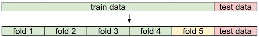
num_folds = 5
k_choices = [1, 3, 5, 8, 10, 12, 15, 20, 50, 100]

X_train_folds = []
y_train_folds = []

X_train_folds = np.array_split(X_train, num_folds)
y_train_folds = np.array_split(y_train, num_folds)

k_to_accuracies = {}

for k in k_choices:
    k_to_accuracies[k] = np.zeros(num_folds)
    for i in range(num_folds):
        Xtr = np.array(X_train_folds[:i] + X_train_folds[i+1:])
        ytr = np.array(y_train_folds[:i] + y_train_folds[i+1:])
        Xte = np.array(X_train_folds[i])
        yte = np.array(y_train_folds[i])

        Xtr = np.reshape(Xtr, (X_train.shape[0] * 4 / 5, -1))
        ytr = np.reshape(ytr, (y_train.shape[0] * 4 / 5, -1))
        Xte = np.reshape(Xte, (X_train.shape[0] / 5, -1))
        yte = np.reshape(yte, (y_train.shape[0] / 5, -1))

        classifier.train(Xtr, ytr)
        yte_pred = classifier.predict(Xte, k)
        yte_pred = np.reshape(yte_pred, (yte_pred.shape[0], -1))
        num_correct = np.sum(yte_pred == yte)
        accuracy = float(num_correct) / len(yte)
        k_to_accuracies[k][i] = accuracy
# Print out the computed accuracies
for k in sorted(k_to_accuracies):
    for accuracy in k_to_accuracies[k]:
        print ('k = %d, accuracy = %f' % (k, accuracy))
OUTPUT:
k = 1, accuracy = 0.263000
k = 1, accuracy = 0.257000
k = 1, accuracy = 0.264000
k = 1, accuracy = 0.278000
k = 1, accuracy = 0.266000
k = 3, accuracy = 0.241000
k = 3, accuracy = 0.249000
k = 3, accuracy = 0.243000
k = 3, accuracy = 0.273000
k = 3, accuracy = 0.264000
k = 5, accuracy = 0.258000
k = 5, accuracy = 0.273000
k = 5, accuracy = 0.281000
k = 5, accuracy = 0.290000
k = 5, accuracy = 0.272000
k = 8, accuracy = 0.263000
k = 8, accuracy = 0.288000
k = 8, accuracy = 0.278000
k = 8, accuracy = 0.285000
k = 8, accuracy = 0.277000
k = 10, accuracy = 0.265000
k = 10, accuracy = 0.296000
k = 10, accuracy = 0.278000
k = 10, accuracy = 0.284000
k = 10, accuracy = 0.286000
k = 12, accuracy = 0.260000
k = 12, accuracy = 0.294000
k = 12, accuracy = 0.281000
k = 12, accuracy = 0.282000
k = 12, accuracy = 0.281000
k = 15, accuracy = 0.255000
k = 15, accuracy = 0.290000
k = 15, accuracy = 0.281000
k = 15, accuracy = 0.281000
k = 15, accuracy = 0.276000
k = 20, accuracy = 0.270000
k = 20, accuracy = 0.281000
k = 20, accuracy = 0.280000
k = 20, accuracy = 0.282000
k = 20, accuracy = 0.284000
k = 50, accuracy = 0.271000
k = 50, accuracy = 0.288000
k = 50, accuracy = 0.278000
k = 50, accuracy = 0.269000
k = 50, accuracy = 0.266000
k = 100, accuracy = 0.256000
k = 100, accuracy = 0.270000
k = 100, accuracy = 0.263000
k = 100, accuracy = 0.256000
k = 100, accuracy = 0.263000
# plot the raw observations
for k in k_choices:
  accuracies = k_to_accuracies[k]
  plt.scatter([k] * len(accuracies), accuracies)

# plot the trend line with error bars that correspond to standard deviation
accuracies_mean = np.array([np.mean(v) for k,v in sorted(k_to_accuracies.items())])
accuracies_std = np.array([np.std(v) for k,v in sorted(k_to_accuracies.items())])
plt.errorbar(k_choices, accuracies_mean, yerr=accuracies_std)
plt.title('Cross-validation on k')
plt.xlabel('k')
plt.ylabel('Cross-validation accuracy')
plt.show()
OUTPUT:

基於交叉驗證集選出合適的K值
# Based on the cross-validation results above, choose the best value for k,
# retrain the classifier using all the training data, and test it on the test
# data. You should be able to get above 28% accuracy on the test data.
best_k = 5
classifier = KNearestNeighbor()
classifier.train(X_train, y_train)
y_test_pred = classifier.predict(X_test, k=best_k)

# Compute and display the accuracy
num_correct = np.sum(y_test_pred == y_test)
accuracy = float(num_correct) / num_test
print ('Got %d / %d correct => accuracy: %f' % (num_correct, num_test, accuracy))
#>>Got 142 / 500 correct => accuracy: 0.284000