
CNN——識別手勢小專案
本文來自Coursera深度學習系列課程專案作業,請勿作為商業用途使用。
需要資料集的可以郵箱聯絡我 [email protected]
Convolutional Neural Networks: Application
Welcome to Course 4’s second assignment! In this notebook, you will:
- Implement helper functions that you will use when implementing a TensorFlow model
- Implement a fully functioning ConvNet using TensorFlow
After this assignment you will be able to:
- Build and train a ConvNet in TensorFlow for a classification problem
We assume here that you are already familiar with TensorFlow. If you are not, please refer the TensorFlow Tutorial of the third week of Course 2 (“Improving deep neural networks“).
1.0 - TensorFlow model
In the previous assignment, you built helper functions using numpy to understand the mechanics behind convolutional neural networks. Most practical applications of deep learning today are built using programming frameworks, which have many built-in functions you can simply call.
As usual, we will start by loading in the packages.
import math
import numpy as np
import h5py
import matplotlib.pyplot as plt
import scipy
from PIL import Image
from scipy import ndimage
import tensorflow as tf
from tensorflow.python.framework import ops
from cnn_utils import *

%matplotlib inline
np.random.seed(1)
Run the next cell to load the “SIGNS” dataset you are going to use.
# Loading the data (signs)
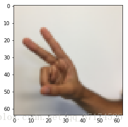
X_train_orig, Y_train_orig, X_test_orig, Y_test_orig, classes = load_dataset()As a reminder, the SIGNS dataset is a collection of 6 signs representing numbers from 0 to 5.

The next cell will show you an example of a labelled image in the dataset. Feel free to change the value of index below and re-run to see different examples.
# Example of a picture
index = 6
plt.imshow(X_train_orig[index])
print ("y = " + str(np.squeeze(Y_train_orig[:, index])))
y = 2
In Course 2, you had built a fully-connected network for this dataset. But since this is an image dataset, it is more natural to apply a ConvNet to it.
To get started, let’s examine the shapes of your data.
X_train = X_train_orig/255.
X_test = X_test_orig/255.
Y_train = convert_to_one_hot(Y_train_orig, 6).T
Y_test = convert_to_one_hot(Y_test_orig, 6).T
print ("number of training examples = " + str(X_train.shape[0]))
print ("number of test examples = " + str(X_test.shape[0]))
print ("X_train shape: " + str(X_train.shape))
print ("Y_train shape: " + str(Y_train.shape))
print ("X_test shape: " + str(X_test.shape))
print ("Y_test shape: " + str(Y_test.shape))
conv_layers = {}
number of training examples = 1080
number of test examples = 120
X_train shape: (1080, 64, 64, 3)
Y_train shape: (1080, 6)
X_test shape: (120, 64, 64, 3)
Y_test shape: (120, 6)
1.1 - Create placeholders
TensorFlow requires that you create placeholders for the input data that will be fed into the model when running the session.
Exercise: Implement the function below to create placeholders for the input image X and the output Y. You should not define the number of training examples for the moment. To do so, you could use “None” as the batch size, it will give you the flexibility to choose it later. Hence X should be of dimension [None, n_H0, n_W0, n_C0] and Y should be of dimension [None, n_y]. Hint.
# GRADED FUNCTION: create_placeholders

def create_placeholders(n_H0, n_W0, n_C0, n_y):
    """
    Creates the placeholders for the tensorflow session.

    Arguments:
    n_H0 -- scalar, height of an input image
    n_W0 -- scalar, width of an input image
    n_C0 -- scalar, number of channels of the input
    n_y -- scalar, number of classes

    Returns:
    X -- placeholder for the data input, of shape [None, n_H0, n_W0, n_C0] and dtype "float"
    Y -- placeholder for the input labels, of shape [None, n_y] and dtype "float"
    """

    ### START CODE HERE ### (≈2 lines)
    X = tf.placeholder(tf.float32,shape=(None,n_H0, n_W0, n_C0))
    Y = tf.placeholder(tf.float32,shape=(None,n_y))
    ### END CODE HERE ###

    return X, Y
X, Y = create_placeholders(64, 64, 3, 6)
print ("X = " + str(X))
print ("Y = " + str(Y))X = Tensor("Placeholder_2:0", shape=(?, 64, 64, 3), dtype=float32)
Y = Tensor("Placeholder_3:0", shape=(?, 6), dtype=float32)
Expected Output
| X = Tensor(“Placeholder:0”, shape=(?, 64, 64, 3), dtype=float32) |
| Y = Tensor(“Placeholder_1:0”, shape=(?, 6), dtype=float32) |
1.2 - Initialize parameters
You will initialize weights/filters and using tf.contrib.layers.xavier_initializer(seed = 0). You don’t need to worry about bias variables as you will soon see that TensorFlow functions take care of the bias. Note also that you will only initialize the weights/filters for the conv2d functions. TensorFlow initializes the layers for the fully connected part automatically. We will talk more about that later in this assignment.
Exercise: Implement initialize_parameters(). The dimensions for each group of filters are provided below. Reminder - to initialize a parameter of shape [1,2,3,4] in Tensorflow, use:
W = tf.get_variable("W", [1,2,3,4], initializer = ...)# GRADED FUNCTION: initialize_parameters
def initialize_parameters():
"""
Initializes weight parameters to build a neural network with tensorflow. The shapes are:
W1 : [4, 4, 3, 8]
W2 : [2, 2, 8, 16]
Returns:
parameters -- a dictionary of tensors containing W1, W2
"""
tf.set_random_seed(1) # so that your "random" numbers match ours
### START CODE HERE ### (approx. 2 lines of code)
W1 = tf.get_variable("W1",[4,4,3,8],initializer=tf.contrib.layers.xavier_initializer(seed=0))
W2 = tf.get_variable("W2",[2,2,8,16],initializer=tf.contrib.layers.xavier_initializer(seed=0))
### END CODE HERE ###
parameters = {"W1": W1,
"W2": W2}
return parameterstf.reset_default_graph()
with tf.Session() as sess_test:
parameters = initialize_parameters()
init = tf.global_variables_initializer()
sess_test.run(init)
print("W1 = " + str(parameters["W1"].eval()[1,1,1]))
print("W2 = " + str(parameters["W2"].eval()[1,1,1]))W1 = [ 0.00131723 0.14176141 -0.04434952 0.09197326 0.14984085 -0.03514394
-0.06847463 0.05245192]
W2 = [-0.08566415 0.17750949 0.11974221 0.16773748 -0.0830943 -0.08058
-0.00577033 -0.14643836 0.24162132 -0.05857408 -0.19055021 0.1345228
-0.22779644 -0.1601823 -0.16117483 -0.10286498]
* Expected Output:*
| W1 = |
[ 0.00131723 0.14176141 -0.04434952 0.09197326 0.14984085 -0.03514394 -0.06847463 0.05245192] |
| W2 = |
[-0.08566415 0.17750949 0.11974221 0.16773748 -0.0830943 -0.08058 -0.00577033 -0.14643836 0.24162132 -0.05857408 -0.19055021 0.1345228 -0.22779644 -0.1601823 -0.16117483 -0.10286498] |
1.2 - Forward propagation
In TensorFlow, there are built-in functions that carry out the convolution steps for you.
tf.nn.conv2d(X,W1, strides = [1,s,s,1], padding = ‘SAME’): given an input and a group of filters , this function convolves ’s filters on X. The third input ([1,f,f,1]) represents the strides for each dimension of the input (m, n_H_prev, n_W_prev, n_C_prev). You can read the full documentation here
tf.nn.max_pool(A, ksize = [1,f,f,1], strides = [1,s,s,1], padding = ‘SAME’): given an input A, this function uses a window of size (f, f) and strides of size (s, s) to carry out max pooling over each window. You can read the full documentation here
tf.nn.relu(Z1): computes the elementwise ReLU of Z1 (which can be any shape). You can read the full documentation here.
tf.contrib.layers.flatten(P): given an input P, this function flattens each example into a 1D vector it while maintaining the batch-size. It returns a flattened tensor with shape [batch_size, k]. You can read the full documentation here.
tf.contrib.layers.fully_connected(F, num_outputs): given a the flattened input F, it returns the output computed using a fully connected layer. You can read the full documentation here.
In the last function above (tf.contrib.layers.fully_connected), the fully connected layer automatically initializes weights in the graph and keeps on training them as you train the model. Hence, you did not need to initialize those weights when initializing the parameters.
Exercise:
Implement the forward_propagation function below to build the following model: CONV2D -> RELU -> MAXPOOL -> CONV2D -> RELU -> MAXPOOL -> FLATTEN -> FULLYCONNECTED. You should use the functions above.
In detail, we will use the following parameters for all the steps:
- Conv2D: stride 1, padding is “SAME”
- ReLU
- Max pool: Use an 8 by 8 filter size and an 8 by 8 stride, padding is “SAME”
- Conv2D: stride 1, padding is “SAME”
- ReLU
- Max pool: Use a 4 by 4 filter size and a 4 by 4 stride, padding is “SAME”
- Flatten the previous output.
- FULLYCONNECTED (FC) layer: Apply a fully connected layer without an non-linear activation function. Do not call the softmax here. This will result in 6 neurons in the output layer, which then get passed later to a softmax. In TensorFlow, the softmax and cost function are lumped together into a single function, which you’ll call in a different function when computing the cost.
# GRADED FUNCTION: forward_propagation

def forward_propagation(X, parameters):
    """
    Implements the forward propagation for the model:
    CONV2D -> RELU -> MAXPOOL -> CONV2D -> RELU -> MAXPOOL -> FLATTEN -> FULLYCONNECTED

    Arguments:
    X -- input dataset placeholder, of shape (input size, number of examples)
    parameters -- python dictionary containing your parameters "W1", "W2"
                  the shapes are given in initialize_parameters

    Returns:
    Z3 -- the output of the last LINEAR unit
    """

    # Retrieve the parameters from the dictionary "parameters"
    W1 = parameters['W1']
    W2 = parameters['W2']

    ### START CODE HERE ###
    # CONV2D: stride of 1, padding 'SAME'
    Z1 = tf.nn.conv2d(X,W1,strides=[1,1,1,1],padding="SAME")
    # RELU
    A1 = tf.nn.relu(Z1)
    # MAXPOOL: window 8x8, sride 8, padding 'SAME'
    P1 = tf.nn.max_pool(A1,ksize=[1,8,8,1],strides=[1,8,8,1],padding="SAME")
    # CONV2D: filters W2, stride 1, padding 'SAME'
    Z2 = tf.nn.conv2d(P1,W2,strides=[1,1,1,1],padding="SAME")
    # RELU
    A2 = tf.nn.relu(Z2)
    # MAXPOOL: window 4x4, stride 4, padding 'SAME'
    P2 = tf.nn.max_pool(A2,ksize=[1,4,4,1],strides=[1,4,4,1],padding="SAME")
    # FLATTEN
    P2 = tf.contrib.layers.flatten(P2)
    # FULLY-CONNECTED without non-linear activation function (not not call softmax).
    # 6 neurons in output layer. Hint: one of the arguments should be "activation_fn=None"
    Z3 = tf.contrib.layers.fully_connected(P2,6,activation_fn=None)
    ### END CODE HERE ###

    return Z3
tf.reset_default_graph()
with tf.Session() as sess:
np.random.seed(1)
X, Y = create_placeholders(64, 64, 3, 6)
parameters = initialize_parameters()
Z3 = forward_propagation(X, parameters)
init = tf.global_variables_initializer()
sess.run(init)
a = sess.run(Z3, {X: np.random.randn(2,64,64,3), Y: np.random.randn(2,6)})
print("Z3 = " + str(a))Z3 = [[-0.44670227 -1.57208765 -1.53049231 -2.31013036 -1.29104376 0.46852064]
[-0.17601591 -1.57972014 -1.4737016 -2.61672091 -1.00810647 0.5747785 ]]
Expected Output:
| Z3 = |
[[-0.44670227 -1.57208765 -1.53049231 -2.31013036 -1.29104376 0.46852064] [-0.17601591 -1.57972014 -1.4737016 -2.61672091 -1.00810647 0.5747785 ]] |
1.3 - Compute cost
Implement the compute cost function below. You might find these two functions helpful:
- tf.nn.softmax_cross_entropy_with_logits(logits = Z3, labels = Y): computes the softmax entropy loss. This function both computes the softmax activation function as well as the resulting loss. You can check the full documentation here.
- tf.reduce_mean: computes the mean of elements across dimensions of a tensor. Use this to sum the losses over all the examples to get the overall cost. You can check the full documentation here.
* Exercise*: Compute the cost below using the function above.
# GRADED FUNCTION: compute_cost

def compute_cost(Z3, Y):
    """
    Computes the cost

    Arguments:
    Z3 -- output of forward propagation (output of the last LINEAR unit), of shape (6, number of examples)
    Y -- "true" labels vector placeholder, same shape as Z3

    Returns:
    cost - Tensor of the cost function
    """

    ### START CODE HERE ### (1 line of code)
    cost = tf.reduce_mean(tf.nn.softmax_cross_entropy_with_logits(logits=Z3,labels=Y))
    ### END CODE HERE ###

    return cost
tf.reset_default_graph()
with tf.Session() as sess:
np.random.seed(1)
X, Y = create_placeholders(64, 64, 3, 6)
parameters = initialize_parameters()
Z3 = forward_propagation(X, parameters)
cost = compute_cost(Z3, Y)
init = tf.global_variables_initializer()
sess.run(init)
a = sess.run(cost, {X: np.random.randn(4,64,64,3), Y: np.random.randn(4,6)})
print("cost = " + str(a))cost = 2.91034
Expected Output:
| cost = | 2.91034 |
1.4 Model
Finally you will merge the helper functions you implemented above to build a model. You will train it on the SIGNS dataset.
You have implemented random_mini_batches() in the Optimization programming assignment of course 2. Remember that this function returns a list of mini-batches.
Exercise: Complete the function below.
The model below should:
- create placeholders
- initialize parameters
- forward propagate
- compute the cost
- create an optimizer
Finally you will create a session and run a for loop for num_epochs, get the mini-batches, and then for each mini-batch you will optimize the function. Hint for initializing the variables
# GRADED FUNCTION: model

def model(X_train, Y_train, X_test, Y_test, learning_rate = 0.009,
          num_epochs = 100, minibatch_size = 64, print_cost = True):
    """
    Implements a three-layer ConvNet in Tensorflow:
    CONV2D -> RELU -> MAXPOOL -> CONV2D -> RELU -> MAXPOOL -> FLATTEN -> FULLYCONNECTED

    Arguments:
    X_train -- training set, of shape (None, 64, 64, 3)
    Y_train -- test set, of shape (None, n_y = 6)
    X_test -- training set, of shape (None, 64, 64, 3)
    Y_test -- test set, of shape (None, n_y = 6)
    learning_rate -- learning rate of the optimization
    num_epochs -- number of epochs of the optimization loop
    minibatch_size -- size of a minibatch
    print_cost -- True to print the cost every 100 epochs

    Returns:
    train_accuracy -- real number, accuracy on the train set (X_train)
    test_accuracy -- real number, testing accuracy on the test set (X_test)
    parameters -- parameters learnt by the model. They can then be used to predict.
    """

    ops.reset_default_graph()                         # to be able to rerun the model without overwriting tf variables
    tf.set_random_seed(1)                             # to keep results consistent (tensorflow seed)
    seed = 3                                          # to keep results consistent (numpy seed)
    (m, n_H0, n_W0, n_C0) = X_train.shape
    n_y = Y_train.shape[1]
    costs = []                                        # To keep track of the cost

    # Create Placeholders of the correct shape
    ### START CODE HERE ### (1 line)
    X, Y = create_placeholders( n_H0, n_W0, n_C0,n_y)
    ### END CODE HERE ###

    # Initialize parameters
    ### START CODE HERE ### (1 line)
    parameters = initialize_parameters()
    ### END CODE HERE ###

    # Forward propagation: Build the forward propagation in the tensorflow graph
    ### START CODE HERE ### (1 line)
    Z3 = forward_propagation(X,parameters)
    ### END CODE HERE ###

    # Cost function: Add cost function to tensorflow graph
    ### START CODE HERE ### (1 line)
    cost = compute_cost(Z3,Y)
    ### END CODE HERE ###

    # Backpropagation: Define the tensorflow optimizer. Use an AdamOptimizer that minimizes the cost.
    ### START CODE HERE ### (1 line)
    optimizer = tf.train.AdamOptimizer(learning_rate).minimize(cost)
    ### END CODE HERE ###

    # Initialize all the variables globally
    init = tf.global_variables_initializer()

    # Start the session to compute the tensorflow graph
    with tf.Session() as sess:

        # Run the initialization
        sess.run(init)

        # Do the training loop
        for epoch in range(num_epochs):

            minibatch_cost = 0.
            num_minibatches = int(m / minibatch_size) # number of minibatches of size minibatch_size in the train set
            seed = seed + 1
            minibatches = random_mini_batches(X_train, Y_train, minibatch_size, seed)

            for minibatch in minibatches:

                # Select a minibatch
                (minibatch_X, minibatch_Y) = minibatch
                # IMPORTANT: The line that runs the graph on a minibatch.
                # Run the session to execute the optimizer and the cost, the feedict should contain a minibatch for (X,Y).
                ### START CODE HERE ### (1 line)
                _ , temp_cost = sess.run([optimizer,cost],feed_dict={X:minibatch_X,Y:minibatch_Y})
                ### END CODE HERE ###

                minibatch_cost += temp_cost / num_minibatches


            # Print the cost every epoch
            if print_cost == True and epoch % 5 == 0:
                print ("Cost after epoch %i: %f" % (epoch, minibatch_cost))
            if print_cost == True and epoch % 1 == 0:
                costs.append(minibatch_cost)


        # plot the cost
        plt.plot(np.squeeze(costs))
        plt.ylabel('cost')
        plt.xlabel('iterations (per tens)')
        plt.title("Learning rate =" + str(learning_rate))
        plt.show()

        # Calculate the correct predictions
        predict_op = tf.argmax(Z3, 1)
        correct_prediction = tf.equal(predict_op, tf.argmax(Y, 1))

        # Calculate accuracy on the test set
        accuracy = tf.reduce_mean(tf.cast(correct_prediction, "float"))
        print(accuracy)
        train_accuracy = accuracy.eval({X: X_train, Y: Y_train})
        test_accuracy = accuracy.eval({X: X_test, Y: Y_test})
        print("Train Accuracy:", train_accuracy)
        print("Test Accuracy:", test_accuracy)

        return train_accuracy, test_accuracy, parameters
Run the following cell to train your model for 100 epochs. Check if your cost after epoch 0 and 5 matches our output. If not, stop the cell and go back to your code!
_, _, parameters = model(X_train, Y_train, X_test, Y_test)Cost after epoch 0: 1.917929
Cost after epoch 5: 1.506757
Cost after epoch 10: 0.955359
Cost after epoch 15: 0.845802
Cost after epoch 20: 0.701174
Cost after epoch 25: 0.571977
Cost after epoch 30: 0.518435
Cost after epoch 35: 0.495806
Cost after epoch 40: 0.429827
Cost after epoch 45: 0.407291
Cost after epoch 50: 0.366394
Cost after epoch 55: 0.376922
Cost after epoch 60: 0.299491
Cost after epoch 65: 0.338870
Cost after epoch 70: 0.316400
Cost after epoch 75: 0.310413
Cost after epoch 80: 0.249549
Cost after epoch 85: 0.243457
Cost after epoch 90: 0.200031
Cost after epoch 95: 0.175452
Expected output: although it may not match perfectly, your expected output should be close to ours and your cost value should decrease.
| **Cost after epoch 0 =** | 1.917929 |
| **Cost after epoch 5 =** | 1.506757 |
| **Train Accuracy =** | 0.940741 |
| **Test Accuracy =** | 0.783333 |
Congratulations! You have finised the assignment and built a model that recognizes SIGN language with almost 80% accuracy on the test set. If you wish, feel free to play around with this dataset further. You can actually improve its accuracy by spending more time tuning the hyperparameters, or using regularization (as this model clearly has a high variance).
Once again, here’s a thumbs up for your work!
fname = "images/thumbs_up.jpg"
image = np.array(ndimage.imread(fname, flatten=False))
my_image = scipy.misc.imresize(image, size=(64,64))
plt.imshow(my_image)
相關推薦
CNN——識別手勢小專案
本文來自Coursera深度學習系列課程專案作業,請勿作為商業用途使用。 需要資料集的可以郵箱聯絡我 [email protected] Convolutional Neural Networks: Application Welcome to
通用物體識別小專案
#用來進行百度雲身份驗證 from aip import AipImageClassify def client(): """ 你的 APPID AK SK """ APP_ID = '' API_KEY = '' SECRET_KEY = '' retu
如何用卷積神經網路CNN識別手寫數字集BaseLine版本 超級小白註釋
如何用卷積神經網路CNN識別手寫數字集? 由於剛剛開始學習機器學習方面的知識,網上很多基礎的教程真的看不懂,所以只能自己一點點摸索,一篇很簡單的程式碼,可能我也要看很久QAQ,原博主的程式碼對於我來說可能還是很懵逼,因此自己加了很多註釋,希望可以幫到和我一樣的
TensorFlow框架做實時人臉識別小專案(二)
在第一部分中,分析了整個小專案的體系,重點討論了用於人臉檢測對齊的mtcnn網路的實現原理,並利用膝上型電腦自帶的攝像頭進行了測試。今天在這裡要討論的重點是人臉識別中的核心部分——facenet網路。facenet是Google開源的人臉識別框架,它的作用是把輸入的人臉影象對
python資料分析練手小專案-汽車銷售偷漏納稅人識別
本專案主要掌握資料預處理和神經網路、決策樹建模以及利用roc曲線進行模型評價。 import pandas as pd data=pd.read_excel(data/cardata.xls',index_col=0) #資料探索 import matp
TensorFlow框架做實時人臉識別小專案(一)
人臉識別是深度學習最有價值也是最成熟的的應用之一。在研究環境下,人臉識別已經趕上甚至超過了人工識別的精度。一般來說,一個完整的人臉識別專案會包括兩大部分:人臉檢測與人臉識別。下面就我近期自己練習寫的一個“粗糙”的人臉識別小專案講起,也算是做一個學習記錄。首先 ,整個專案的框架
Kinect 常用識別手勢
swiper spa 微軟 原版 out 1.5 wip 手勢 down 以下手勢能被流暢的識別: ◎RaiseRightHand / RaiseLeftHand – 左手或右手舉起過肩並保持至少一秒 ◎Psi –雙手舉起過肩並保持至少一秒 ◎Stop – 雙手下垂. ◎W
生物特征識別:小面積指紋識別算法(二)
dpi 如果 mage 卷積 噪聲 狀態 AMM 計算 log 算法(一)已經介紹了一種小面積指紋識別算法可選的方案,是一種經典的方案,對於面積足夠大且level2特征高於最小限制時,為一種低內存占用,快速的實現方法。但在某些應用場中中(比如終端中,要求占用面積較小,且面
C語言小專案——註釋轉換
我們要測試幾種情況,將一些.c檔案裡的C語言註釋轉換成c++語言註釋。 commentconvert.h #ifndef __COMMENTCONVERT_H__ #define __COMMENTCONVERT_H__ #include<stdio.h> #include<
VUE小專案問題之用axios外掛取本地json檔案,報404錯誤。
一、問題 在用axios獲取本地json資料時,總是報404錯誤。 百思不得其解。 二、經過 看網友們都是把本地json檔案放在static檔案中。 我寫的專案存放在assets中,恍然大悟,應該是檔案位置。 三、結果 檔案改存為static axios({
class 2-3 小專案練習
空氣質量分指數計算方法(框架) 1 def cal_liner(iaqi_lo,iaqi_hi,bp_lo,bp_hi,cp): 2 """範圍縮放""" 3 iaqi =(iaqi_hi - iaqi_lo)*(cp -bp_lo) /(bp_hi - bp_l
記一次Android選修的小專案
目標和思路 目標: 做一個有多級頁面的app,使用者選擇需要選擇的資訊:性別、年齡、姓名。點選提交,會根據隨機生成一個三國時期的人物與其對應。並提示相關資訊。 思路: 編寫多個頁面,通過intent元件實現頁面跳轉,並在MainActivity.class檔案中根據選項的選擇
小專案(Gensim庫)--維基百科中文資料處理
1.下載維基百科資料 https://dumps.wikimedia.org/zhwiki/latest/ 2.預處理檔案:將壓縮的檔案轉化成.txt檔案 新增指令碼檔案process.py,程式碼如下: import logging import os.path import sys
小專案(文字資料分析)--新聞分類任務
1.資料 import pandas as pd import jieba #資料(一小部分的新聞資料) df_news = pd.read_table('val.txt',names=['category','theme','URL','content'],encoding='ut
小專案--貝葉斯實現拼寫檢查
求解:argmaxc P(c|w) -> argmaxc P(w|c)P©/P(w) P©:文章中出現一個正確拼寫詞c的概率,也就是語料庫中c出現的概率有多大 P(w|c):在使用者想鍵入c的情況下敲成w的概率,也就是使用者會以多大的概率把c敲錯成w argmaxc:用來列舉所有可能的
簡單Java類和資料庫操作及javafx的結合小專案
先圖為上 秦時明月漢時關,萬里長征人未還,妙呀,甚是.. 1.開始 1.專案目的: 開發工具: Idea + Mysql + JAVASE 1.其實簡單來說就是實現兩張資料表的基本操作, 1.新增 2. 刪除 3.修改
class 2-2 小專案練習
一. 判斷第幾天 閏年(四年一閏,百年不閏,四百年再閏) 元組(tuple) 用於表達固定資料項、函式多返回值等 特點: 1.元素可以是不同型別(元組通常不同資料組成,列表通常由相同型別資料組成) 2.元組中各元素存在先後關係,可通過索引訪問元組中元素(元組表示的是結構,列表表示的是順序)
上班簽到小專案(nodejs,express,ajax)
效果圖 express配合客戶端ajax實現上班簽到小專案(資料庫部分暫時省略,使用虛擬資料) 簡單需求分析: 1.使用者(id,name,password) 2.使用者必須登入才能簽到 3.使用者從哪裡來,註冊(暫時存到陣列) 4.簽到(誰,時間,地
Java資料庫小專案
0 JDBC的簡單使用 1 package Test; 2 3 import java.sql.Connection; 4 import java.sql.Driver; 5 import java.sql.DriverManager; 6 import java.sql.DriverP
第一階段基本結束,獨自完成了一個小專案。雖然還有許多不足,但自己依舊在進步!加油!!!!
package com.jbit.sms; /** * 學生資訊管理系統 * @author Administrator * */ import java.util.Arrays; import java.util.Scanner; impor