A guide to convolution arithmetic for deep learning
一、Discrete convolutions
A discrete convolution is a linear transformation that preserves this notion of ordering. It is sparse (only a few input units contribute to a given output unit) and reuses parameters (the same weights are applied to multiple locations in the input).
The bread and butter of neural networks is affine transformations
: a vector is received as input and is multiplied with a matrix to produce an output (to which a bias vector is usually added before passing the result through a nonlinearity). This is applicable to any type of input, be it an image, a sound clip or an unordered collection of features: whatever their dimensionality, their representation can always be flattened into a vector before the transformation.Images, sound clips and many other similar kinds of data have an intrinsic structure. More formally, they share these important properties:
They are stored as multi-dimensional arrays.
They feature one or more axes for which ordering matters (e.g., width and height axes for an image, time axis for a sound clip).
One axis, called the channel axis, is used to access different views of the data (e.g., the red, green and blue channels of a color image, or the left and right channels of a stereo audio track).
二、Pooling
In some sense, pooling works very much like a discrete convolution, but replaces the linear combination described by the kernel with some other function。
Since pooling does not involve zero padding, the relationship describing the general case is as follows:
三、Convolution arithmetic
1. Same Padding(步長為1,padding 為 kernel_size/2 向下取整的值)
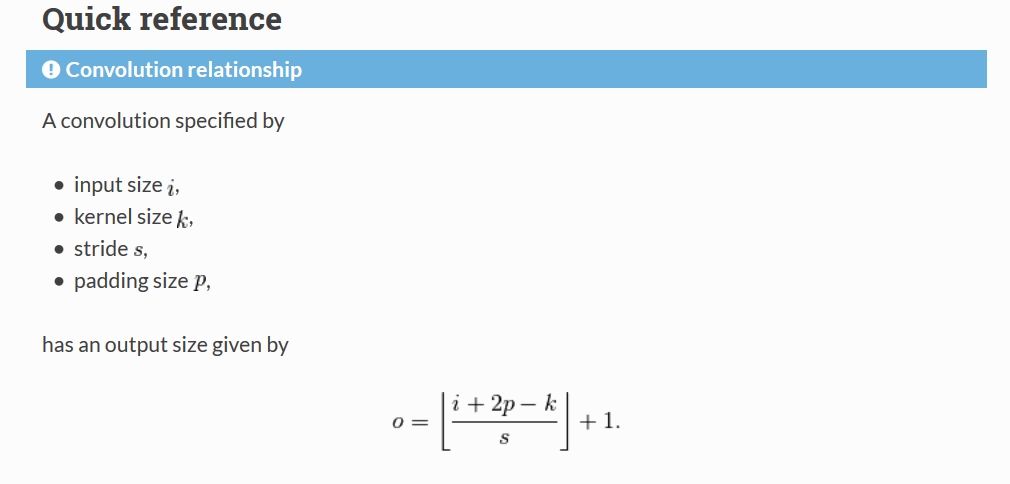
2. Convolution Relationship
四、Transposed convolution arithmetic
Since every convolution boils down to an efficient implementation of a matrix operation, the insights gained from the fully-connected case are useful in solving the convolutional case.
1. Convolution as a matrix operation
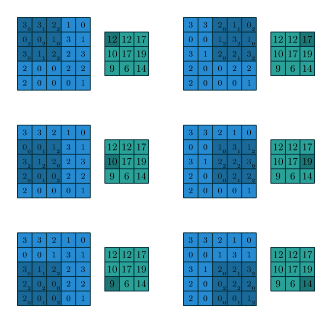
Take for example the convolution presented in the No zero padding, unit strides subsection:
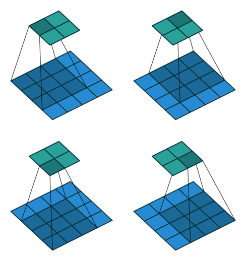
If the input and output were to be unrolled into vectors from left to right, top to bottom, the convolution could be represented as a sparse matrix

This linear operation takes the input matrix flattened as a 16-dimensional vector and produces a 4-dimensional vector that is later reshaped as the
輸入矩陣可展開為16維向量,記作x
輸出矩陣可展開為4維向量,記作y
卷積運算可表示為y = Cx
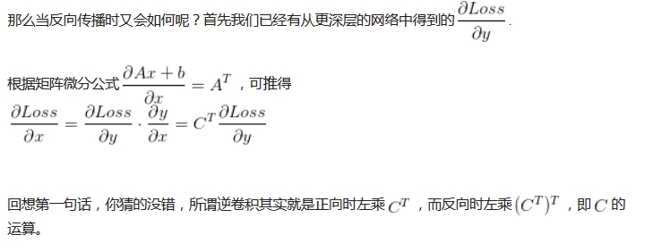
Using this representation, the backward pass is easily obtained by transposing
Notably, the kernel
2. Transposed convolution
Transposed convolutions – also called fractionally strided convolutions – work by swapping the forward and backward passes of a convolution. One way to put it is to note that the kernel defines a convolution, but whether it’s a direct convolution or a transposed convolution is determined by how the forward and backward passes are computed.
The transposed convolution operation can be thought of as the gradient of some convolution with respect to its input, which is usually how transposed convolutions are implemented in practice.
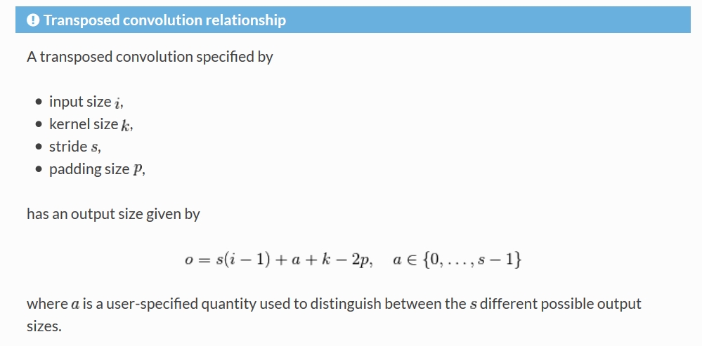
3. Transposed convolution relationship

