RBF網路能夠逼近任意非線性的函式。可以處理系統內難以解析的規律性，具有很好的泛化能力，並且具有較快的學

習速度。當網路的一個或多個可調引數（權值或閾值）對任何一個輸出都有影響時，這樣的網路稱為全域性逼近網路。

由於對於每次輸入，網路上的每一個權值都要調整，從而導致全域性逼近網路的學習速度很慢，比如BP網路。如果對於

輸入空間的某個區域性區域只有少數幾個連線權值影響輸出，則該網路稱為區域性逼近網路，比如RBF網路。接下來重點

先介紹RBF網路的原理，然後給出其實現。先看如下圖

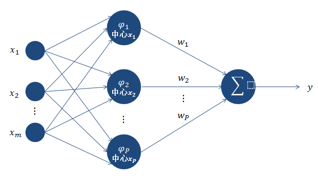
 正則化的RBF網路參考這裡。下面是網上找的一個比較好的Python的RBF網路實現。

程式碼：

from scipy import *
from scipy.linalg import norm, pinv
 
from matplotlib import pyplot as plt
 
class RBF:
     
    def __init__(self, indim, numCenters, outdim):
        self.indim = indim
        self.outdim = outdim
        self.numCenters = numCenters
        self.centers = [random.uniform(-1, 1, indim) for i in xrange(numCenters)]
        self.beta = 8
        self.W = random.random((self.numCenters, self.outdim))
         
    def _basisfunc(self, c, d):
        assert len(d) == self.indim
        return exp(-self.beta * norm(c-d)**2)
     
    def _calcAct(self, X):
        # calculate activations of RBFs
        G = zeros((X.shape[0], self.numCenters), float)
        for ci, c in enumerate(self.centers):
            for xi, x in enumerate(X):
                G[xi,ci] = self._basisfunc(c, x)
        return G
     
    def train(self, X, Y):
        """ X: matrix of dimensions n x indim 
            y: column vector of dimension n x 1 """
         
        # choose random center vectors from training set
        rnd_idx = random.permutation(X.shape[0])[:self.numCenters]
        self.centers = [X[i,:] for i in rnd_idx]
         
        print "center", self.centers
        # calculate activations of RBFs
        G = self._calcAct(X)
        print G
         
        # calculate output weights (pseudoinverse)
        self.W = dot(pinv(G), Y)
         
    def test(self, X):
        """ X: matrix of dimensions n x indim """
         
        G = self._calcAct(X)
        Y = dot(G, self.W)
        return Y
 
      
if __name__ == '__main__':
    n = 100
    x = mgrid[-1:1:complex(0,n)].reshape(n, 1)
    # set y and add random noise
    y = sin(3*(x+0.5)**3 - 1)
    # y += random.normal(0, 0.1, y.shape)
     
    # rbf regression
    rbf = RBF(1, 10, 1)
    rbf.train(x, y)
    z = rbf.test(x)
       
    # plot original data
    plt.figure(figsize=(12, 8))
    plt.plot(x, y, 'k-')
     
    # plot learned model
    plt.plot(x, z, 'r-', linewidth=2)
     
    # plot rbfs
    plt.plot(rbf.centers, zeros(rbf.numCenters), 'gs')
     
    for c in rbf.centers:
        # RF prediction lines
        cx = arange(c-0.7, c+0.7, 0.01)
        cy = [rbf._basisfunc(array([cx_]), array([c])) for cx_ in cx]
        plt.plot(cx, cy, '-', color='gray', linewidth=0.2)
     
    plt.xlim(-1.2, 1.2)
    plt.show()
    
 

最後提供Github上的一個，供日後參考。