本週你將使用k-均值聚類演算法和主成分分析法。

一、k-均值聚類

k-均值將用於影象壓縮。你將先在2維的資料集上開始來幫助我們理解k-均值是怎麼運作的。你將通過減少顏色的數目來進行壓縮。

（1）k-均值

k-均值的演算法是一種自動的進行聚類相似的資料集的演算法。提供給你一組訓練集，你需要將他們分成相似的組。k-均值的本質是一種迭代演算法，開始先隨機初始化中心點，然後不斷地通過給樣本賦值他們的中心點是離他們最近的點，然後通過賦值重新計算中心點。 演算法如下：

%Initialize centroids
centroids=kMeansInitCentroids(X,K);
for iter=1:iterations
    %Cluster assignment step:Assign each data point to the closest
    %cebtroid.idx(i) corresponds to c^(i),the index of the centroid
    %assigned to example i
    idx=findClosestCentroids(X,centroids);
    %move centroid step:Compute means based on centroid
    %assignments
    centroids=computeMeans(X,idx,K);
end
 

最後我們的k-均值會到一個最後的中心點的平均值，注意最後的結果不一定是好的，取決於k-均值的初始化。所以最好的方法是多次隨機初始化，然後選擇那個使得代價最小的那個。

1.為每個樣本例項找到最佳的中心點

對於每一個樣例，我們設定，指的是離最近的中心點的下標，指的是第j箇中心點的位置，注意我們的程式碼裡面這個idx（i）指的就是現在的。需要你完成findClosestCentroids.m的程式碼。這個函式的功能是接收資料矩陣X和中心點的位置centroids，然後輸出一個一維的陣列idx，裡面的元素在1-K之間，是每一個訓練樣例的最近的中心點下標。你可以為每個樣本和每個中心點設定for迴圈。 程式碼如下：

for i=1:size(X,1)
    idx(i,1)=1
    maxvalue=sum(sum((X(i,:)-centroids(1,:)).^2))
    for j=2:K
        nextvalue=sum(sum((X(i,:)-centroids(j,:)).^2))
        if(nextvalue<maxvalue)
            maxvalue=nextvalue
            idx(i,1)=j
        end
    end
end
 

由這裡輸出idx的樣例，你會發現idx是行向量。

2.計算中心均值

對於每個中心點，你需要使用公式：，是屬於第k箇中心點的樣本的數量。完成computeCentroids.m的程式碼，你可以使用for迴圈，但是如果你可以使用向量化的操作就不需要for迴圈。 第一種方法使用兩個for迴圈：（其實還需要補充一句判斷count等於還是不等於0的操作）

for i=1:K
    count=0;
    for j=1:m
        if(idx(j,1)==i)
            centroids(i,:)=centroids(i,:)+X(j,:);
            count=count+1;
        end
    end
    centroids(i,:)=centroids(i,:)./count;
end
 

第二種方法使用一個for迴圈：idx是一個行向量

for i=1:K  
    if(size(find(idx==i),2)~=0)  
        centroids(i,:)=mean(X(find(idx==i),:));  
    else  
        centroids(i,:)=zeros(1,n);  
    end  
end  

（2）應用k-均值到資料集上

當你完成（1）裡面的兩個函式，ex7.m的程式碼會執行runKmeans.m在2D資料集上應用k-均值。雖然runKmeans.m的程式碼你不需要寫，但是鼓勵你看看。你會看到隨著迭代步數慢慢執行，你可以觀察到這個改變中心點和中心點賦值的過程。 程式碼：

function [centroids, idx] = runkMeans(X, initial_centroids, ...
                                      max_iters, plot_progress)
%RUNKMEANS runs the K-Means algorithm on data matrix X, where each row of X
%is a single example
%   [centroids, idx] = RUNKMEANS(X, initial_centroids, max_iters, ...
%   plot_progress) runs the K-Means algorithm on data matrix X, where each 
%   row of X is a single example. It uses initial_centroids used as the
%   initial centroids. max_iters specifies the total number of interactions 
%   of K-Means to execute. plot_progress is a true/false flag that 
%   indicates if the function should also plot its progress as the 
%   learning happens. This is set to false by default. runkMeans returns 
%   centroids, a Kxn matrix of the computed centroids and idx, a m x 1 
%   vector of centroid assignments (i.e. each entry in range [1..K])
%

% Set default value for plot progress
if ~exist('plot_progress', 'var') || isempty(plot_progress)
    plot_progress = false;
end

% Plot the data if we are plotting progress
if plot_progress
    figure;
    hold on;
end

% Initialize values
[m n] = size(X);
K = size(initial_centroids, 1);
centroids = initial_centroids;
previous_centroids = centroids;
idx = zeros(m, 1);

% Run K-Means
for i=1:max_iters
    
    % Output progress
    fprintf('K-Means iteration %d/%d...\n', i, max_iters);
    if exist('OCTAVE_VERSION')
        fflush(stdout);
    end
    
    % For each example in X, assign it to the closest centroid
    idx = findClosestCentroids(X, centroids);
    
    % Optionally, plot progress here
    if plot_progress
        plotProgresskMeans(X, centroids, previous_centroids, idx, K, i);
        previous_centroids = centroids;
        fprintf('Press enter to continue.\n');
        pause;
    end
    
    % Given the memberships, compute new centroids
    centroids = computeCentroids(X, idx, K);
end

% Hold off if we are plotting progress
if plot_progress
    hold off;
end

end

一次迭代：
。。。 十次迭代：

（3）隨機初始化

每次通過選擇你的樣本來隨機初始化，完成KMeansInitCentroids.m：

%Initialize the centroids to be random examples
%randomly reorder the indices of examples
randidx = randperm(size(X,1));
%Take the first K examples as centroids
centoids=X(randidx(1:K),:);

上面的程式碼：先是使用randperm隨機的改變樣本的下標序列，接著選擇前K個樣本作為中心點。

（4）應用k-均值進行影象壓縮

給我們提供了一個圖形，這個圖形是每一個畫素都是三個8位的數字（0-255）分別代表紅，綠和藍色的密度值（RGB）。我們的影象儲存了上千的顏色，要求將這些顏色減少至16個。你將使用k-均值來選擇這16個顏色，你可以將原本影象裡面的畫素都當做成一個一個的樣本，使用k-均值演算法在三維的RGB空間找到最佳聚類的16個顏色。

在matlab你可以使用下面的程式碼來讀取一個圖形：

%Load 128*128 color image(bird_small.png)
A=imread('bird_samll.png');
%You will need to have installed the image package to used imread. If you
%do not have the image package installed, you should instead change the
%following line to 
%load('bird_small.mat');%loads the image into the variable A

這個創造了一個三維的矩陣A，A的前兩個下標指明瞭畫素的位置，下一個下標代表的是紅，綠還是藍。例如（20,33,3）給了20行33列的畫素密度。

在ex7.m的程式碼load了這個圖形，改變他的大小變成一個m*3的畫素顏色矩陣（m=16384=128*128），然後運用k-均值。

A = A / 255; % Divide by 255 so that all values are in the range 0 - 1

% Size of the image
img_size = size(A);

% Reshape the image into an Nx3 matrix where N = number of pixels.
% Each row will contain the Red, Green and Blue pixel values
% This gives us our dataset matrix X that we will use K-Means on.
X = reshape(A, img_size(1) * img_size(2), 3);

當你得到了最佳的16個顏色來代表這個影象，你可以將每個畫素賦值成離自己最近的中心點使用函式findClosestCentoids.m。原始的影象需要24位元來表示128*128個畫素地位置，導致需要128*128*24=393,216位元。縮短之後需要的總的儲存空間是：128*128*4+16*24=65,920bits，16個顏色，每一個需要24bits，每個畫素需要4bits來儲存畫素的位置。

（5）使用你自己的影象（附加題）

在這個練習中，我們修改程式碼運用到我們自己的影象上。注意，如果你的影象很大，k-均值會花很長的時間。因此建議你，給你的影象重新規定大小，你也可以改變K值看看壓縮的影響。 我直接修改的是ex7.m的程式碼：把自己的影象放到包下，完成下面的程式碼即可，有點慢

%  Load an image of a bird
A = double(imread('shen.jpg'));

% If imread does not work for you, you can try instead

%%load ('bird_small.mat');


shen=imread('shen.jpg');
save shen;
load('shen.mat');


A = A / 255; % Divide by 255 so that all values are in the range 0 - 1

% Size of the image
img_size = size(A);

% Reshape the image into an Nx3 matrix where N = number of pixels.
% Each row will contain the Red, Green and Blue pixel values
% This gives us our dataset matrix X that we will use K-Means on.
X = reshape(A, img_size(1) * img_size(2), 3);

% Run your K-Means algorithm on this data
% You should try different values of K and max_iters here
K = 16; 
max_iters = 10;

% When using K-Means, it is important the initialize the centroids
% randomly. 
% You should complete the code in kMeansInitCentroids.m before proceeding
initial_centroids = kMeansInitCentroids(X, K);

% Run K-Means
[centroids, idx] = runkMeans(X, initial_centroids, max_iters);

fprintf('Program paused. Press enter to continue.\n');
pause;


%% ================= Part 5: Image Compression ======================
%  In this part of the exercise, you will use the clusters of K-Means to
%  compress an image. To do this, we first find the closest clusters for
%  each example. After that, we 

fprintf('\nApplying K-Means to compress an image.\n\n');

% Find closest cluster members
idx = findClosestCentroids(X, centroids);

% Essentially, now we have represented the image X as in terms of the
% indices in idx. 

% We can now recover the image from the indices (idx) by mapping each pixel
% (specified by its index in idx) to the centroid value
X_recovered = centroids(idx,:);

% Reshape the recovered image into proper dimensions
X_recovered = reshape(X_recovered, img_size(1), img_size(2), 3);

% Display the original image 
subplot(1, 2, 1);
imagesc(A); 
title('Original');

% Display compressed image side by side
subplot(1, 2, 2);
imagesc(X_recovered)
title(sprintf('Compressed, with %d colors.', K));


fprintf('Program paused. Press enter to continue.\n');
pause;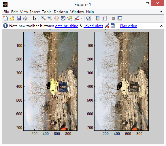

二、主成分分析法

（1）樣例

我們先從2維的資料開始，看看PCA是怎麼樣執行的，將二維資料降維到一維的資料。

（2）應用PCA

step0：在開始PCA之前最好進行歸一化資料（featureNormalize.m之前的部落格介紹過） 下面的兩個步驟包含在pca.m裡面，你需要完成上面的程式碼： step1：計算協方差矩陣：，Sigma是一個n*n維的矩陣，不是求和操作 step2：svd函式來計算特徵向量：[U,S,V]=svd(Sigma),S是一個對角矩陣，而U包含主成分。 輸出的特徵向量即主成分的結果可能是[0.707,0.707]或者[-0.707,-0.707] 程式碼如下：Returns the eigenvectors U, the eigenvalues (on diagonal) in S

Sigma=X'*X/m;
[U,S,V]=svd(Sigma);

（3）應用PCA進行降維

1.將資料投影到主成分上

完成projectData.m的程式碼：給定了資料集X和主成分U還有K。你將資料投影到U中的前K個主成分： 結果可能是正負1.481！ 程式碼如下：

Ureduce=U(:,1:K);
Z=X*Ureduce;%X是m*n維，Ureduce是n*k維，得到的z是m*k維

2.重建資料的近似值

當你將資料投影到更低維，你可以通過將它映射回原來的維度來換還原你的資料。你需要完成REcoverData.m的程式碼：將Z中的樣例映射回原來的空間，返回原資料的近似X_rec。結果是[-1.047,-1.047]。 程式碼如下：

Ureduce=U(:,1:K);%Ureduce->n*K,Z=m*K要求得到的X_rec->m*n
X_rec=Z*Ureduce';

3.視覺化投影

當你完成上面的兩個程式碼，ex7_pca.m將會演示投影和重建資料的過程。原資料是藍色的圈，而投影出來的低維的資料是紅色的。

（4）人臉影象資料集-ex7faces.mat包含X的人臉資料集，每一個都是32*32維度的灰色影象。每一行是一個人臉的影象，大小是1024。

1.人臉上的PCA

step0：歸一化 step1：PCA 當運行了PCA之後，你會得到資料集的主成分，U中的每一個主成分，每一行都是一個n維的向量，代表了人臉資料集n=1024。我們可以視覺化主成分，通過reshape每一個向量成為一個32*32維度的矩陣。ex7_pac.m展示了前36個主成分。

2.降維

前面你已經得到了資料集的主成分，現在你可以使用它來完成降維的工作。降低到100維，前100個主成分。每一張臉原本是1024維度，現在只有100維度。當你完成這樣的降維到100的操作之後，在完成重建的操作會出現下圖：（所以說但你使用神經網路進行人臉識別的時候，可以進行降維加速你的學習演算法）

（5）視覺化方面的PCA應用（附加題）

在之前的k-均值的影象壓縮的練習裡面，我們使用K-均值演算法在一個3維的RGB空間。在之後的ex7_pca.m裡面，ng為我們提供了scatter3的功能來實現視覺化最後的畫素賦值。每一個數據點都被染色了，通過他所屬於的聚類。你可以通過你的滑鼠來旋轉觀察結果。

之後我們的ex7_pac.m將這個三維的資料降維到2維平面（scatter來繪製scatter影象）