如何讓孩子愛上機器學習？

1. 梯度

gradient f : ▽f = (  ∂f/∂x, ∂f/∂x, ∂f/∂x )

a) 這是一個向量

b) 偏導和普通導數的區別就在於對x求偏導的時候，把y z 看成是常數  （對y求偏導就把x z 看成是常數）

梯度方向其實就是函式增長方向最快的地方，梯度的大小代表了這個速率究竟有多大，因此在迭代的過程中，我們有兩種選擇：

向著梯度方向前進->梯度上升

向著梯度反方向前進->梯度下降

需要注意的是，梯度本身是一個極限的區域性概念，所以我們在更新的時候應該要較小範圍的進行更新，否則可能會因為步長太大的原因並沒有得到我們想要的下降結果，所以我們一般會引入一個學習率引數 α 來控制更新的速度

2. 引數解釋

Andrew NG 在第一講裡引入了一些引數的約定，在這裡寫一下

1. 訓練樣本(training example)數m： 在後來的程式碼實現裡通常也是DataMatrix的行數（m個樣本）

2. 特徵(feature)數n：每個樣本所擁有的特徵的數量。 例如一個房子擁有：面積，臥室數兩個特徵，我們說 n = 2

3.我們約定指數是樣本次序，而右下角的腳標是樣本的特徵次序

4. 假設函式hθ （X）表示以x為變數，θ為引數的函式，是我們學習得到的一個預測函式

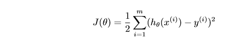
5. 為了度量引數好壞，引入損失函式，這個函式只有一個極小值點，所以這個點也是全域性最小值

3. 梯度下降

梯度下降可以分成隨機梯度下降和批梯度下降兩種。

批梯度下降每次更新引數的時候都用到了訓練集中所有的樣本，這樣使得每一次更新迭代進行的計算量很大，特別是當m:特別大的時候，更新的速度會很慢，以前用matlab實現的時候程式碼寫的不是很好，每一個迴圈裡還有符號計算，導致迭代速度非常慢，所以個人其實不是很喜歡批梯度下降...

直接上兩個實現的例子，隨機梯度是以前從csdn文章裡大概抄下來的實現程式，然後我修改了一下改成了批梯度下降

# _*_ coding: utf-8 _*_  
# 批梯度下降
x = [(1, 0., 3), (1, 1., 3), (1, 3., 2), (1, 4., 4)]
#y = [95.364, 97.217205, 75.195834, 60.105519, 49.342380]
y = [10, 12, 13, 21]
eps = 0.00000001

alpha = 0.01
diff = [0, 0, 0]
max_itor = 1000
error1 = 0
error0 = 0
count = 0
m = len(x)


theta0 = 0
theta1 = 0
theta2 = 0

	
while True:
	count += 1
	# 更新梯度	
	diff[0] = diff[1] = diff[2] = 0
	for i in range(m):	# += 是因為這是對所有樣本進行一次更新，J(θ)和隨機梯度下降是不一樣的
		diff[0] += ((theta0 + theta1 * x[i][1] + theta2 * x[i][2]) - y[i]) * 1
		diff[1] += ((theta0 + theta1 * x[i][1] + theta2 * x[i][2]) - y[i]) * x[i][1]
		diff[2] += ((theta0 + theta1 * x[i][1] + theta2 * x[i][2]) - y[i]) * x[i][2]

	# 更新梯度 for all j simultaneously
	theta0 -= alpha * diff[0]
	theta1 -= alpha * diff[1]
	theta2 -= alpha * diff[2]

	error1 = 0
	for i in range(m):
		error1 += 1/2 *(y[i] - theta0 - theta1 * x[i][1] - theta2 * x[i][2]) ** 2
	if abs(error1 - error0) < eps:
		break
	else:
		error0 = error1

	print(' theta0 : %f, theta1 : %f, theta2 : %f, error1 : %f' % (theta0, theta1, theta2, error1))  
	print('Done: theta0 : %f, theta1 : %f, theta2 : %f' % (theta0, theta1, theta2))
	print('迭代次數: %d' % count)
 

# _*_ coding: utf-8 _*_  

#隨機梯度下降

x = [(1, 0., 3), (1, 1., 3), (1, 3., 2), (1, 4., 4)]
#y = [95.364, 97.217205, 75.195834, 60.105519, 49.342380]
y = [10, 12, 13, 21]
eps = 0.0000000001

alpha = 0.001
diff = [0, 0]
max_itor = 1000
error1 = 0
error0 = 0
count = 0
m = len(x)


theta0 = 0
theta1 = 0
theta2 = 0
	
while True:
	count += 1

	for i in range(m):
		diff[0] = (theta0 + theta1 * x[i][1] + theta2 * x[i][2]) - y[i]

		theta0 -= alpha * diff[0]
		theta1 -= alpha * diff[0] * x[i][1]
		theta2 -= alpha * diff[0] * x[i][2]
	error1 = 0
	for lp in range(m):
		error1 += (y[lp]-(theta0 + theta1 * x[lp][1] + theta2 * x[lp][2]))**2/2  
	if abs(error1 - error0) < eps:
		break
	else:
		error0 = error1
	print(' theta0 : %f, theta1 : %f, theta2 : %f, error1 : %f' % (theta0, theta1, theta2, error1))  
	print('Done: theta0 : %f, theta1 : %f, theta2 : %f' % (theta0, theta1, theta2))
	print('迭代次數: %d' % count)