一維常係數對流方程的學習——來自流沙公眾號

認識：
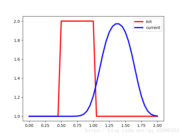
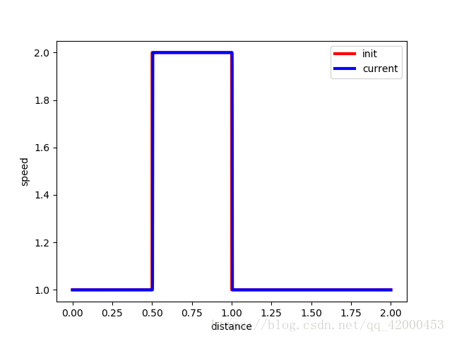
1、時間步長越小越靠後移動；網格越小則波的形狀越一致,波形失真在減小，引出Courant數：u*dt/dx<sigma；
2、對numpy中的ones（）、linspace（）、zeros（）有基礎認識；
3、再次練習了matplotlib中的pyplot。
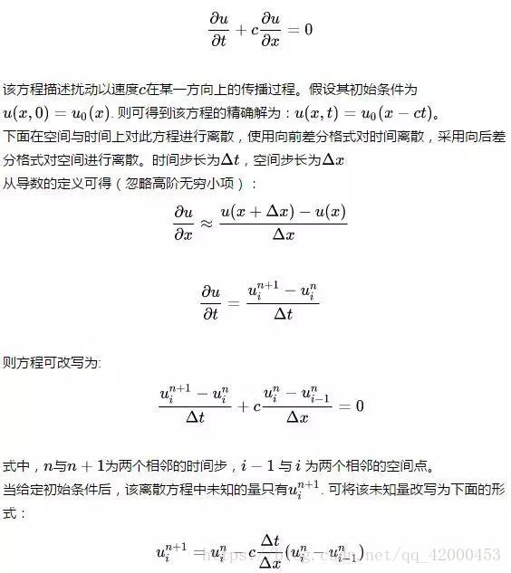
4、明白了一維方程程式設計的簡單運算，基礎

import numpy as np
# numpy是Python的一個科學計算的庫，提供了矩陣運算的功能，其一般與Scipy、matplotlib一起使用。
import matplotlib.pyplot as plt

def linearconv(nx):
	dx = 2/(nx - 1) # 空間網格步長，x方向總長度為2
	nt = 25 # 總的時間步長
	sigma = 0.8  # Courant數
	c = 1 # 常數
	dt =  sigma * dx / c  # 時間步長

	# 指定初始條件
	u = np.ones(nx)
	u[int(0.5/dx):int(1/dx + 1)] = 2 # 這一行實際上是製造了一個方波(0.5--1)
	# 下面將初始條件畫出來
	plt.plot(np.linspace(0,2,nx),u,'r',linewidth=3,label = 'init') # linspace用於產生x1,x2之間的N點行向量,其中x1、x2、N分別為起始值、終止值、元素個數

	# 計算25個時間步後的波長
	un = np.ones(nx)
	for n in range(nt):
		un = u.copy() # 後面的計算會改變u，故將u拷貝到un
		for i in range(1,nx):
			u[i] = un[i] - c * dt / dx * (un[i] - un[i-1])

	plt.plot(np.linspace(0,2,nx),u,'b',linewidth = 3, label = 'current')
	plt.xlabel("distance")
	plt.ylabel("speed")
	plt.legend()
	plt.show()

linearconv(10001)
# 時間步長越小越靠後移動；網格越小則波的形狀越一致,波形失真在減小，故引出了Courant數：u*dt/dx<sigma