
大叔學ML第四:線性迴歸正則化
目錄
正則:正則是一個漢語詞彙,拼音為zhèng zé,基本意思是正其禮儀法則;正規;常規;正宗等。出自《楚辭·離騷》、《插圖本中國文學史》、《東京賦》等文獻。 —— 百度百科
基本形式
線性迴歸模型常常會出現過擬合的情況,由於訓練集噪音的干擾,訓練出來的模型抖動很大,不夠平滑,導致泛化能力差,如下所示:
import numpy as np
import matplotlib.pyplot as plt
from sklearn.preprocessing import PolynomialFeatures

def poly4(X, *theta):
    return theta[0] + theta[1] * X + theta[2] * X**2 + theta[3] * X**3 + theta[4] * X**4

''' 建立樣本資料 '''
X = np.arange(0, 9, 1)
Y = [-10, 1, 10, 19, 10, 10, 46, 49, 50]

''' 用4次多項式擬合 '''
pf = PolynomialFeatures(degree=4)
featrues_matrix = pf.fit_transform(X.reshape(9, 1))

theta = tuple(np.dot(np.dot(np.linalg.pinv(np.dot(featrues_matrix.T, featrues_matrix)), featrues_matrix.T), np.array(Y).T))
Ycalculated = poly4(X, *theta)

plt.scatter(X, Y, marker='x', color='k')
plt.plot(X, Ycalculated, color='r')
plt.show()
執行結果:
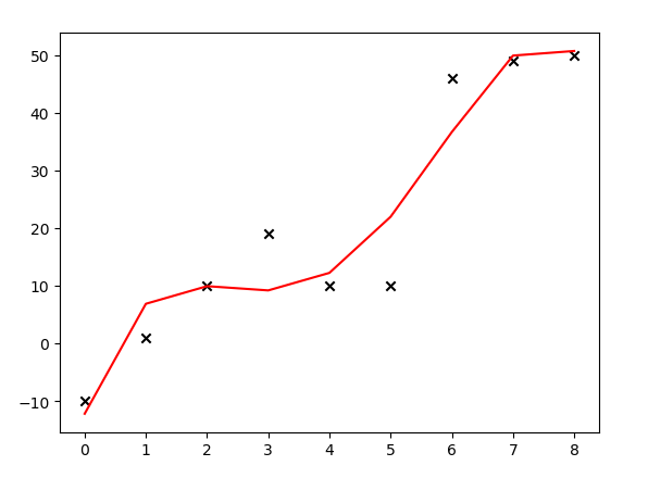
上面的程式碼中,大叔試圖用多項式\(\theta_0 + \theta_1x + \theta_2x^2 + \theta_3x^3 + \theta_4x^4\)擬合給出的9個樣本(如對以上程式碼有疑問,可參見大叔學ML第三:多項式迴歸),用正規方程計算出\(\vec\theta\),並繪圖發現:模型產生了過擬合的情況。解決線性迴歸過擬合的一個方案是給代價函式新增正則化項。代價函式(參見大叔學ML第二:線性迴歸)形如:
\[j(\theta_0,\theta_1\dots \theta_n)=\frac{1}{2m}\sum_{k=1}^m (\theta_0x_0^{(k)} + \theta_1 x_1^{(k)} + \theta_2 x_2^{(k)} + \dots + \theta_n x_n^{(k)} - y^{(k)})^2 \tag{1}\]
新增正則化後的代價函式形如:
\[j(\theta_0,\theta_1\dots \theta_n)=\frac{1}{2m}\left[\sum_{k=1}^m (\theta_0x_0^{(k)} + \theta_1 x_1^{(k)} + \theta_2 x_2^{(k)} + \dots + \theta_n x_n^{(k)} - y^{(k)})^2 +\lambda\sum_{i=0}^n \theta_i^2 \tag{2}\right]\],其中\(\lambda > 0\)。直觀地理解:當我們不加正則化項時,上面的程式碼擬合出來的多項式某些項前面的係數\(\theta\)
梯度下降法中應用正則化項
對(2)式中的\(\vec\theta\)求偏導:
- \(\frac{\partial}{\partial\theta_0}j(\theta_0,\theta_1\dots \theta_n) = \frac{1}{m}\left[\sum_{k=1}^m(\theta_0x_0^{(k)} + \theta_1x_1^{(k)} + \dots+ \theta_nx_n^{(k)} - y^{(k)})x_0^{(k)} + \lambda\theta_0\right]\)
- \(\frac{\partial}{\partial\theta_1}j(\theta_0,\theta_1\dots \theta_n) = \frac{1}{m}\left[\sum_{k=1}^m(\theta_0x_0^{(k)} + \theta_1x_1^{(k)} + \dots+ \theta_nx_n^{(k)}- y^{(k)})x_1^{(k)} + \lambda\theta_1\right]\)
- \(\dots\)
- \(\frac{\partial}{\partial\theta_n}j(\theta_0,\theta_1\dots \theta_n) = \frac{1}{m}\left[\sum_{k=1}^m(\theta_0x_0^{(k)} + \theta_1x_1^{(k)} + \dots+ \theta_nx_n^{(k)}- y^{(k)})x_n^{(k)} + \lambda\theta_n\right]\)
有了偏導公式後修改原來的程式碼(參見大叔學ML第二:線性迴歸)即可,不再贅述。
正規方程中應用正則化項
用向量的形式表示代價函式如下:
\[J(\vec\theta)=\frac{1}{2m}||X\vec\theta - \vec{y}||^2 \tag{3}\]
觀察(2)式,添加了正則化項的向量表示形式如下:
\[J(\vec\theta)=\frac{1}{2m}\left[||X\vec\theta - \vec{y}||^2 + \lambda||\vec\theta||^2\right] \tag{4}\]
變形:
\[\begin{align} J(\vec\theta)&=\frac{1}{2m}\left[||X\vec\theta - \vec{y}||^2 + ||\vec\theta||^2\right] \\ &=\frac{1}{2m}\left[(X\vec\theta - \vec{y})^T(X\vec\theta - \vec{y}) + \lambda\vec\theta^T\vec\theta \right]\\ &=\frac{1}{2m}\left[(\vec\theta^TX^T - \vec{y}^T)(X\vec\theta - \vec{y}) + \lambda\vec\theta^T\vec\theta\right] \\ &=\frac{1}{2m}\left[(\vec\theta^TX^TX\vec\theta - \vec\theta^TX^T\vec{y}- \vec{y}^TX\vec\theta + \vec{y}^T\vec{y}) + \lambda\vec\theta^T\vec\theta\right]\\ &=\frac{1}{2m}(\vec\theta^TX^TX\vec\theta - 2\vec{y}^TX\vec\theta + \vec{y}^T\vec{y} + \lambda\vec\theta^T\vec\theta)\\ \end{align}\]
對\(\vec\theta\)求導:
\[\begin{align} \frac{d}{d\vec\theta}J(\vec\theta)&=\frac{1}{m}(X^TX\vec\theta-X^T\vec{y} + \lambda I\vec\theta) \\ \frac{d}{d\vec\theta}J(\vec\theta)&=\frac{1}{m}\left[(X^TX + \lambda I)\vec\theta-X^T\vec{y}\right] \end{align}\]
令其等於0,得:\[\vec\theta=(X^TX + \lambda I)^{-1}X^T\vec{y}\tag{5}\]
小試牛刀
對本文開頭所給出的程式碼進行修改,加入正則化項看看效果:
import numpy as np
import matplotlib.pyplot as plt
from sklearn.preprocessing import PolynomialFeatures

def poly4(X, *theta):
    return theta[0] + theta[1] * X + theta[2] * X**2 + theta[3] * X**3 + theta[4] * X**4

''' 建立樣本資料 '''
X = np.arange(0, 9, 1)
Y = [-10, 1, 10, 19, 10, 10, 46, 49, 50]

''' 用4次多項式擬合 '''
pf = PolynomialFeatures(degree=4)
featrues_matrix = pf.fit_transform(X.reshape(9, 1))

ReM = np.eye(5) #正則化矩陣
ReM[0, 0] = 0

theta1 = tuple(np.dot(np.dot(np.linalg.pinv(np.dot(featrues_matrix.T, featrues_matrix) + 0 * ReM), featrues_matrix.T), np.array(Y).T))
Y1 = poly4(X, *theta1)

theta2 = tuple(np.dot(np.dot(np.linalg.pinv(np.dot(featrues_matrix.T, featrues_matrix) + 1 * ReM), featrues_matrix.T), np.array(Y).T))
Y2 = poly4(X, *theta2)

theta3 = tuple(np.dot(np.dot(np.linalg.pinv(np.dot(featrues_matrix.T, featrues_matrix) + 10000 * ReM), featrues_matrix.T), np.array(Y).T))
Y3 = poly4(X, *theta3)

plt.scatter(X, Y, marker='x', color='k')
plt.plot(X, Y1, color='r')
plt.plot(X, Y2, color='y')
plt.plot(X, Y3, color='b')

plt.show()
執行結果:
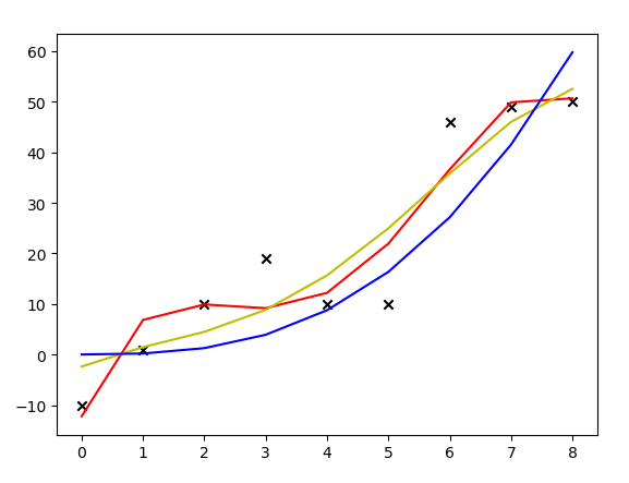
上圖中,紅線是沒有加正則化項擬合出來的多項式曲線,黃線是加了\(\lambda\)取1的正則化項後擬合出來的曲線,藍線是加了\(\lambda\)取10000的正則化項擬合出來的曲線。可見,加了正則化項後,模型的抖動變小了,曲線變得更加平滑。
呼叫類庫
sklean中已經為我們寫好了加正則化項的線性迴歸方法,修改上面的程式碼:
import numpy as np
import matplotlib.pyplot as plt
from sklearn.linear_model import Ridge
from sklearn.preprocessing import PolynomialFeatures

def poly4(X, *theta):
    return theta[0] + theta[1] * X + theta[2] * X**2 + theta[3] * X**3 + theta[4] * X**4

''' 建立樣本資料 '''
X = np.arange(0, 9, 1)
Y = [-10, 1, 10, 19, 10, 10, 46, 49, 50]

''' 用4次多項式擬合 '''
pf = PolynomialFeatures(degree=4)
featrues_matrix = pf.fit_transform(X.reshape(9, 1))

ridge_reg = Ridge(alpha=100)
ridge_reg.fit(featrues_matrix, np.array(Y).reshape((9, 1)))
theta = tuple(ridge_reg.intercept_.tolist() + ridge_reg.coef_[0].tolist())

Y1 = poly4(X, *theta)

plt.scatter(X, Y, marker='x', color='k')
plt.plot(X, Y1, color='r')

plt.show()
執行結果:
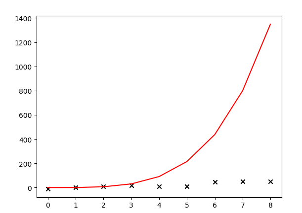
哇,調庫和自己寫程式碼搞出的模型差距居然這麼大。看來水很深啊,大叔低估了ML的難度,路漫漫其修遠兮......將來如果有機會需要閱讀一下這些庫的原始碼。大叔猜測是和樣本數量可能有關係,大叔的樣本太少,自己瞎上的。園子裡高人敬請在評論區指教哦。
擴充套件
正則化項不僅如本文一種新增方式,本文所用的加\(\lambda||\vec\theta||^2\)的方式被稱為“嶺迴歸”,據說是因為給矩陣\(X^TX\)加了一個對角矩陣,此對角矩陣的主元看起來就像一道分水嶺,所以叫“嶺迴歸”。程式碼中用的sklean中的模組名字就是Ridge,也是分水嶺的意思。
除了嶺迴歸,還有“Lasso迴歸”,這個迴歸演算法所用的正則化項是\(\lambda||\vec\theta||\),嶺迴歸的特點是縮小樣本屬性對應的各項\(\theta\),而Lasso迴歸的特點是使某些不打緊的屬性對應的\(\theta\)為0,即:忽略掉了某些屬性。還有一種迴歸方式叫做“彈性網路”,是一種對嶺迴歸和Lasso迴歸的綜合應用。大叔在以後的日子研究好了還會專門再寫一篇博文記錄。
通過這幾天的研究,大叔發現其實ML中最重要的部分就是線性迴歸,連高大上的深度學習也是對線性迴歸的擴充套件,如果對線性迴歸有了透徹的瞭解,定能在ML的路上事半功倍,一往無前。祝大家聖誕快樂!