The above figures show the filters from few intermediate convolution and ReLU layers respectively from InceptionV3 network. I captured these images by running the trained model on one of the test images.

If you take a look at the different images from Convolution layers filters, its pretty clear to see how different filters in different layers are trying to highlight or activate different parts of the image. Some filters are acting as edge detectors, others are detecting a particular region of the flower like its central portion and still others are acting as background detectors. Its easier to see this behavior of convolution layers in starting layers, because as you go deeper the pattern captured by the convolution kernel become more and more sparse, so it might be the case that such patterns might not even exist in your image and hence it would not be captured.

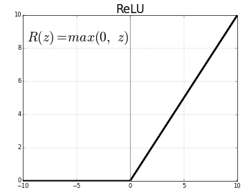
Coming to the ReLU (Rectified Linear Units) activations of corresponding convolution layers, all they do is apply the Relu function to each pixel which is ReLU(z) = max(0, z), as shown in below figure . So, basically, at each pixel the activation function just puts either a 0 or pixel value itself if it is not 0.

By visualizing the output from different convolution layers in this manner, the most crucial thing that you will notice is that the layers that are deeper in the network visualize more training data specific features, while the earlier layers tend to visualize general patterns like edges, texture, background etc. This knowledge is very important when you use Transfer Learning whereby you train some part of a pre-trained network (pre-trained on a different dataset, like ImageNet in this case) on a completely different dataset. The general idea is to freeze the weights of earlier layers, because they will anyways learn the general features, and to only train the weights of deeper layers because these are the layers which are actually recognizing your objects.