Simple Reference Guide for tuning Deep Neural Nets

Getting Started

Designing deep neural nets can be a painful task considering so many parameters involved and no general formula seems to fit all the use cases. We can use CNNs for image classification, LSTMs for NLP related tasks but still number of features, size of features, number of neurons, number of hidden layers, choice of activation functions, initialization of weights etc. will vary for each in different use cases.

These changes in parameters can be attributed to different types of data requires analysis that is independent of other datasets. Like image dataset will have different properties as pixels in neighboring locations are related but in relational database entries can be random with no relation. Hence, a different approach is required for that.

We are able to generalize types of data types and suitable neural network structure for them like CNN for images, audio, video and RNN/LSTMs for NLP related tasks etc. But, to achieve maximum performance out of them we should make them smart. What is smart for neural network ? A neural network that generalize instead of memorize can be attributed as smart neural network. The kind of behavior that is desirable in any form of learning.

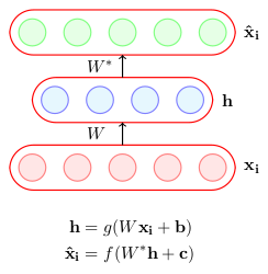
For simplicity in this articles let’s limit discussion to autoencoders, a special type of feed forward neural network which encodes the input in hidden layers and decode from this hidden representation. CNNs are an example of autoencoders for example, CNN classifying digits in MNIST functions in the same way like autoencoders where a network tries to approximate the function of reconstruction of output information from hidden layer. Every neural network architecture is having autoencoders as their basic block. Hence, with discussion on them we can extend the ideas on different deep learning architectures.

In this article we will explore the techniques to fine tune our network for better validation accuracy leading to better predictions. Plus, we will also look into some mathematics behind these techniques to develop an understanding of behind the scenes of these techniques.

What‘ s the issue in creating Smart Autoencoders ?

Well, what we really want from a neural network is to generalize from data available not memorize. The problem with memorization is that the model might end up overfitting. As deep learning models are complex and tend to overfit the target function. Consider very basic case in which models are extensively trained on training dataset such that error on training datset minimizes and approaches zero. It can be possible that neural network instead of capturing trends in data just remembered the way to reproduce whole data with very complex function.

Let’s understand this more clearly using the concept of bias v/s variance trade-off. Have a look at the plot below, the x-axis represents model complexity while the y-axis denotes error. As the complexity increases, the training error tends to decrease, but the variance increases shown with high validation error.

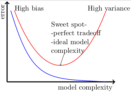
We want models that are more sensitive to change for capturing minute details of sparse but important features. Hence, underfitting the data is not an option at all. As more complex models are more sensitive to changes. Only carrying on discussion about overfitting makes sense in Deep Learning’s context.

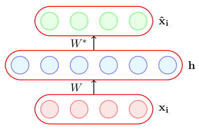
For example take the case of overcomplete autoencoders, in such a case they can learn simple trivial encoding of copy pasting the values throughout the network. Like copying input(xi) onto hidden layer(h) and then again from h to output layer(xhat). Clearly, error will be minimum but there is no learning ?

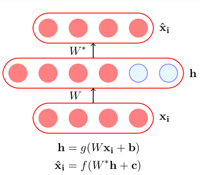
Let’s build upon the idea of above discussion that in order for deep learning autoencoders to be successful overfitting must be removed. Surely, there are also other problems like not having enough data, large number of parameters ,relevant features are learnt or not, when to stop training. From here we can say that smart autoencoders are the ones which generalize the information from which we can observe and learn important trends from which they are able to make predictions. Let’s start exploring these techniques with an aim to develop intuition for reasons to use them and suitable examples along the way to augment our learning.

1. Dataset Augmentation
2. Early Stopping
3. l2 Regularization
4. Avoiding Vanilla Autoencoders: Noise & Sparsity
5. Parameter Sharing & Tying
6. Ensemble Methods to DropOut & DropConnect

Dataset Augmentation

In computer vision classification tasks the model learns better with more training data. But the problem with with huge data is that it increase the training time.

Well, number of parameters in deep learning models are huge(order of million). It will clearly help if you don’t have enough data available at the first place to get started with. But, will it be helpful if you already have enough data ? Yes, as it will increase relevant features in your dataset which helps autoencoders to learn important sparse features as compared to irrelevant abundant ones.

Data augmentation is a technique with which we create new data from existing data with an aim to increase relevant features in our original data. See, illustration below to get an idea about data augmentation.

Augmenting in this way the most obvious features for classification becomes the most relevant ones. Where to augment our data in ML pipeline ? First is Offline augmentation apply transformations and add images to dataset. But, it increases the size by a scale of number of transformations applied. Second, is Online augmentation is applied on mini-batches just before feeding onto our learning model. Here, see some Tensorflow scripts for such transformations applied with an assumptions that we are not concerned whats outside boundary of images.

Now, what does that mean ? Let’s say some part of image has nothing i.e. it is unknown space then we need different transformations as follow. Example, some rotated image with black background.

Tensorflow scripts based on above assumptions on applying simple transformations of data on mini-batches.

# 1. Flip: 'x' = A placeholder for an image.shape = [height, width, channels]x = tf.placeholder(dtype = tf.float32, shape = shape)flip_2 = tf.image.flip_up_down(x)flip_5 = tf.image.random_flip_left_right(x)

# 2. Rotate: 'y' = A batch of images# To rotate in any angle. In the example below, 'angles' is in radiansshape = [batch, height, width, 3]y = tf.placeholder(dtype = tf.float32, shape = shape)rot_tf_180 = tf.contrib.image.rotate(y, angles=3.1415)

# 3. Noise: 'x' = A placeholder for an image.shape = [height, width, channels]x = tf.placeholder(dtype = tf.float32, shape = shape)

# Adding Gaussian noisenoise = tf.random_normal(shape=tf.shape(x), mean=0.0, stddev=0.5,dtype=tf.float32)output = tf.add(x, noise)

Other augmentation can similarly be written for random cropping, wrapping, color channel shifting etc.

Early Stopping

As name suggests it does gives us some idea that we are avoiding overfitting by stopping early while training. But how early to stop ? Basically, our aim will be to stop before training error is driven towards zero and validation error is about to blown up.

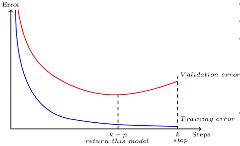
These early stopping rules work by splitting the original training set into a new training set and a validation set. The error on the validation set is used as substitute for original training error in determining when overfitting has begun. With Keras you can simply do this with following method.

keras.callbacks.EarlyStopping(monitor='val_loss',                              min_delta=0,                              patience=0,                              verbose=0, mode='auto')

min_delta is a threshold to whether quantify a loss at some epoch as improvement or not. If the difference of loss is below min_delta, it is quantified as no improvement. Better to leave it as 0 since we're interested in when loss becomes worse.patience argument represents the number of epochs before stopping once your loss starts to increase (stops improving). mode argument depends on what direction your monitored quantity has (is it supposed to be decreasing or increasing), since we monitor the loss, we can use min.

Now, What if I say early stopping is also a type of regularization technique. Can prove this statement to be true ? Let’s see small amount of mathematics to understand the behind the seen working of early stopping. Remember, regularization is any technique which add some constraints on weight & biases in a learning neural network.

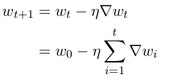
Early stopping stopping allows only t updates of parameters. The more important is the dimension more large will be the loss related to it, as with above equations we control learning rate and t. Only loss related to gradient remains as dominating factor, which effectively mean only important parameters with more loss will account more. Where as, less important will not be able to grow. Hence, important parameters are scaled up which will lead to better accuracy. This is similar to L2 regularization, refer below.

L2 Regularization

Regularization is a constraint that is assigned to a model while learning. L2 regularization is weight decay regularization that drives weights closer to origin with scaling down less important features more.

Let’s understand the concept of true error in intuitive manner. This error can be represented in this given form below, where terms added to empirical error are on the basis of estimation procedure as we don’t know f(x).

Main aim is to link model complexity’s influence on true error. Clearly, it will train error plus something. What’s that something ? With Stein’s Lemma and some mathematics we can prove that

Is this related to complex models ? Yes, the above observation is linked to the fact that more complex the model the more it is sensitive to changes in observations. Hence, we can say that true error = empirical train error + small constant + Ω(model complexity). This Ω is the basis for regularization. Hence, in regularization our aim is to minimize error due to model complexity which in turn is related to bias-variance trade-off.

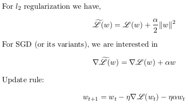
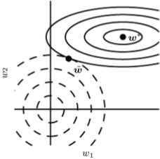
What’s the meaning of above getting added onto update rule and SGD’s formula. Equation two operation mentioned above mathematically signifies scaling of weights matrix in the direction of significance i.e. the one with major eigen values and minor ones gets scaled downed but less important features gets scaled down more. This regularization operation effectively first rotate the weight matrix, then diagonalize it and then again rotate it. Here, see these operations in effect on a contour map diagram. Refer this article for contour maps, read that part only.

Here, is Tensorflow script for using regularization in your neural network model based on above formulas. First illustration is using it on one layer only and second is using it on all the layers.

# Code 1:# Loss function using L2 Regularizationregularizer = tf.nn.l2_loss(weights)loss = tf.reduce_mean(loss + beta * regularizer)# Optimizer. optimizer = tf.train.GradientDescentOptimizer(0.5).minimize(loss)

# Code 2:#Loss for all trainable variables, 0.001 is beta abovevars   = tf.trainable_variables() regularizer = tf.add_n([ tf.nn.l2_loss(v) for v in vars ]) * 0.001# Let's say you wan't to regularize biasesregularizer = tf.add_n([ tf.nn.l2_loss(v) for v in vars                    if 'bias' not in v.name ]) * 0.001

# More descriptive coderegularizers = tf.nn.l2_loss(weights_1) + tf.nn.l2_loss(weights_2) + tf.nn.l2_loss(weights_3) + tf.nn.l2_loss(weights_4) +         tf.nn.l2_loss(weights_5) + tf.nn.l2_loss(weights_6)

loss = tf.reduce_mean(loss + beta * regularizers)

Avoid Vanilla Autoencoders: Noise & Sparsity

Consider the case of overcomplete vanilla autoencoders as mentioned above. Clearly, they are prone to overfitting and trivial learning. Hence, using these Vanilla autoencoders won’t do much good specifically in these cases. One way to resolve this by adding noise to inputs which will force the neural networks not to learn trivial encoding instead focus more generalizations.

# Generate corrupted MNIST images by adding noise with normal dist                       # centered at 0.618 and std=0.618 noise = np.random.normal(loc=0.618, scale=0.618, size=x_train.shape)x_train_noisy = x_train + noise

noise = np.random.normal(loc=0.618, scale=0.618, size=x_test.shape)x_test_noisy = x_test + noise

# np.clip to move out of bound values inside given intervalx_train_noisy = np.clip(x_train_noisy, 0., 1.)                       x_test_noisy = np.clip(x_test_noisy, 0., 1.)

With addition of Gaussian noise these hidden neurons becomes edge detectors, PCA can’t give these edge detectors. Also, noise can be applied on target classes which will result in soft targets with stochastic analysis instead of hard target.

Sparse autoencoders are also used to resolve such issue with sparsity parameters, which will lead to firing of neuron in rare case when the features are relevant to be observed. Can be written as Lˆ(θ) = L(θ) + Ω(θ) where L (θ) is the squared error loss or cross entropy loss and Ω(θ) is the sparsity constraint which forces to trigger neurons for important features.

Bonus: Contractive Autoencoders, regularization term Ω(θ) = ||J x (h)||^ 2 is the Jacobian of encoder. The (j, l) entry of the Jacobian captures the variation in the output of the lth neuron with a small variation in the jth input. L(θ) — capture important variations in data & Ω(θ) — do not capture variations in data, as Jacobian makes neuron not sensitive to variations. With this trade-off we can capture most important features only. Similar argument can be made for Sparse AE.

Parameter sharing & Tying

Shared weights simply means that use same weight vector to do the convulations. The main motivation for this is limit the number of parameters.

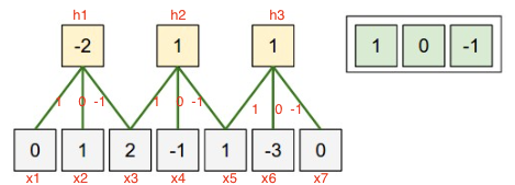
We can dramatically reduce down our parameters by one intuitive assumption that if one feature is important to compute at one point so it is on another point. Example: if detecting an edge is important at particular position. So, it is for all positions that edge repeat itself due to the translationally-invariant structure of images. This will lead to faster convergence. Also, we have limited the flexibility which can also act a regularization mechanism avoiding overfitting. Consider the case where we want to process two sets of images in parallel, but also want columns to share parameters.

def function(x, reuse):  with tf.variable_scope(layer_name) as s:    output = tf.contrib.layers.convolution2d(inputs = x, num_outputs = 10, kernel_size = [3, 3], stride = [1, 1], padding = 'VALID', reuse = reuse, scope = s)  return outputoutput1 = function(image1, False)output2 = function(image2, True)

Weight Tying concept is based on same idea as above with same motivation to reduce down parameters but is applied on autoencoder units in which encoder weight and decoder weights are tied down and used. It reduces the capacity of autoencoder and acts as a regularizer.

Ensemble to DropOut & DropConnect

Ensembles combine outputs for different models to reduce generalization error, models can be different classifiers. Here, they are different instances of same neural network trained on different hyperparameters, features and different samples of training data. Bagging is an approach across entire dataset which trains models on a subset of the training data. Thus some training examples are not shown to a given model. It allows neurons to different neurons to capture different relevant features across training dataset. Error made by average prediction of all models ?

From above, the more independent the models are from each other lesser is the error reducing to (V/k) only. Quite good as the error ideally goes very less when architecture of neural nets vary a lot. But, it explodes the number of training parameters to handle as number of individual models increases. With that training becomes computationally expensive.

Wouldn't it be nice if we could just reduce these parameters. Also, different architectures will help us to increase variance among models. These two problems are solved by Dropout. It gives approximate way of combining many different networks and train several nets w/o any significant overhead. It shares weights among all networks and sample different training network for each training instance. Only, active parameters update from forward and backward propagation. Instead of aggregating 2^n thinned networks, scale the output of each node by the fraction of times it was on during training.

It is applied to features within each training example causing certain features to be unavailable to the network. Because a neuron cannot completely rely on one input, representations in these networks tend to be more distributed and the network is less likely to overfit. This happens as dropout puts masking noise to hidden units which prevents co-adaptation, essentially hidden units won’t rely on others to detect specific features as those unit may get dropped out. This results in hidden units to be more robust.

# Simple keras implementation of MNIST for dropout

import tensorflow as tfmnist = tf.keras.datasets.mnist(x_train, y_train),(x_test, y_test) = mnist.load_data()x_train, x_test = x_train / 255.0, x_test / 255.0model = tf.keras.models.Sequential([  tf.keras.layers.Flatten(),  tf.keras.layers.Dense(512, activation=tf.nn.relu),  tf.keras.layers.Dropout(0.2),  tf.keras.layers.Dense(10, activation=tf.nn.softmax)])model.compile(optimizer='adam',              loss='sparse_categorical_crossentropy',              metrics=['accuracy'])model.fit(x_train, y_train, epochs=5)model.evaluate(x_test, y_test)

What is dropconnect ? Well let’s say instead of dropping nodes we decide to drop subsets of randomly. It will behave in a similar way as dropout. A binary mask drawn from a Bernoulli distribution is applied to the original weight matrix.

Instead of random dropping connections in each training, connections would drop and stay dropped as a result of the input data class or the connection’s contribution to deeper layers.

tf.nn.dropout(W, keep_prob=p) * p ORtf.layers.dropout(W, rate=1-p) * p

Conclusion

The intuition of when to use these techniques in mind we can create effective deep neural networks that are smarter within their core while functioning to learn any specific tasks. We this knowledge in hand we have developed an understanding of creating better deep learning architectures. But, by no means this discussion is complete as along with better accuracy faster convergence is also a desired behavior. Let’s take a look about convergence in follow up article.

Thanks to Aishwarya for improvements. Baseline content is adapted from CS7015(DL) from IITM, great course by Prof. Mitesh M. Khapra . Thanks for reading !!