The very first move: Importing the libraries

from __future__ import print_function
import keras
from keras.datasets import cifar10
from keras.models import Sequential
from keras.layers import Dense, Dropout, Activation, Flatten
from keras.layers import Conv2D, MaxPooling2D
from keras.optimizers import SGD
from keras.utils import print_summary, to_categorical
import sys
import os
 

We need to assign a file path on Google Drive to save the model that we trained on Google Colaboratory. The first thing to do is to create a new folder named “cifar10” on Google Drive and then, let’s run the following code snippet on Google Colab.

sys.path.insert(0, 'drive/cifar10')
os.chdir(“drive/cifar10”)

Initializing the parameters.

We will feed the convolutional neural network with the images as batches -each batch contains 64 images- in 100 epochs and eventually, the network model will output the possibilities of 10 different categories (num_classes) can belong to the image.

batch_size = 64
num_classes = 10
epochs = 100
model_name = 'keras_cifar10_model'
save_dir = '/model/' + model_name
 

Thanks to Keras, we can load the dataset easily.

(x_train, y_train), (x_test, y_test) = cifar10.load_data()

We also need to convert the labels in the dataset into categorical matrix structure from 1-dim numpy array structure.

y_train = to_categorical(y_train, num_classes)
y_test = to_categorical(y_test, num_classes)

Once bitten twice shy, we will not forget it for this time. We need to normalize the images in the dataset.

x_train = x_train.astype('float32')
x_test = x_test.astype('float32')
x_train /= 255.0
x_test /= 255.0

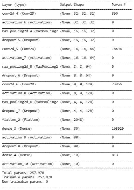
We are now absolutely sure that it is enough for preprocessing -for now, LUL-. It is the time to create our model. For this episode in the series, I would prefer to use the most common neural network model architecture in the literature: [CONV] — [MAXP] -..- [CONV] — [MAXP] — [Dense]

model = Sequential()
model.add(Conv2D(32, (3, 3), padding='same', input_shape=x_train.shape[1:]))
model.add(Activation('relu'))
model.add(MaxPooling2D(pool_size=(2, 2)))
model.add(Dropout(0.3))

model.add(Conv2D(64, (3, 3), padding='same', input_shape=x_train.shape[1:]))
model.add(Activation('relu'))
model.add(MaxPooling2D(pool_size=(2, 2)))
model.add(Dropout(0.3))

model.add(Conv2D(128, (3, 3), padding='same', input_shape=x_train.shape[1:]))
model.add(Activation('relu'))
model.add(MaxPooling2D(pool_size=(2, 2)))
model.add(Dropout(0.4))

model.add(Flatten())
model.add(Dense(80))
model.add(Activation('relu'))
model.add(Dropout(0.3))
model.add(Dense(num_classes))
model.add(Activation('softmax'))

The summary of this model could be seen below:

I would prefer the Stochastic Gradient Descent algorithm to optimize the weights on the backpropagation. Set the momentum parameter as 0.9, and just leave the others as default. I, again, strongly recommend you to read an article, this one, in order to get more information about SGD algorithm.

opt = SGD(lr=0.01, momentum=0.9, decay=0, nesterov=False)

We are now ready to compile our model. The categorical crossentropy function has been picked out as a loss function because we have more than 2 labels and already prepared the labels in the categorical matrix structure -I confess, copied it from the first episode-.

model.compile(loss='categorical_crossentropy',
              optimizer=opt,
              metrics=['accuracy'])

We’ve done a lot and we have only one step to begin training our model. At this time, I would like to make a different move. I will split the training dataset (50.000 images) into training (40.000 images) and validation (10.000 images) datasets to measure the validation accuracy of our model in such a better way. Thus, our neural network model will continue the training by evaluating the images that never been seen during the training after each epoch.

model.fit(x_train, y_train,
          batch_size=batch_size,
          epochs=epochs,
          validation_split=0.2,
          shuffle=True)

Well, so far so good. We have started to learn. I think we did, didn’t we?