From Exploration to Production — Bridging the Deployment Gap for Deep Learning (Part 2)

This is the second part of a series of two blogposts on deep learning model exploration, translation, and deployment. Both involve many technologies like PyTorch, TensorFlow, TensorFlow Serving, Docker, ONNX, NNEF, GraphPipe, and Flask

. We will orchestrate these technologies to solve the task of image classification using the more challenging and less popular EMNIST dataset. In the first part, we introduced EMNIST, developed and trained models with PyTorch, translated them using the Open Neural Network eXchange format (ONNX) and served them through GraphPipe.

This part concludes the series by adding two additional approaches for model deployment. TensorFlow Serving and Docker as well as a rather hobbyist approach in which we build a simple web application that serves our model. Both deployments will offer a REST API to call for predictions. You will find all the related sourcecode on

GitHub. If you like to start from the very beginning, find the first part here on Towards Data Science.

We will use the trained model files from PyTorch and TensorFlow that we generated within the first part. You can find them in the models folder on GitHub.

Model Deployment: TensorFlow Serving and Docker

This is indeed the second time we use TensorFlow Serving within this series. The first time we used it was as part of GraphPipe that among others provides a reference model server and tweaked model server configurations. Instead of using a meta-framework, we now turn to TensorFlow directly. Refer to this JuPyter notebook and follow the steps to experience another way of deep learning model deployment.

As a first step, we have to load our ONNX model and create its TensorFlow representation using the ONNX TensorFlow connector:

Next, we define the path from where to load our model and create a SavedModelBuilder. This instance is required to generate that path and to create a protobuf export of our model. In TensorFlow Serving terminology this specific save path is also called Source.

In order to build a proper signature (some kind of interface) for our model, let’s recap what the model consists of:

External Input: ['flattened_rescaled_img_28x28']External Output: ['softmax_probabilities']

{'weight_1': <tf.Tensor 'Const:0' shape=(512, 784) dtype=float32>, 'bias_1': <tf.Tensor 'Const_1:0' shape=(512,) dtype=float32>, 'weight_2': <tf.Tensor 'Const_2:0' shape=(256, 512) dtype=float32>, 'bias_2': <tf.Tensor 'Const_3:0' shape=(256,) dtype=float32>, 'weight_3': <tf.Tensor 'Const_4:0' shape=(62, 256) dtype=float32>, 'bias_3': <tf.Tensor 'Const_5:0' shape=(62,) dtype=float32>, 'flattened_rescaled_img_28x28': <tf.Tensor 'flattened_rescaled_img_28x28:0' shape=(1, 784) dtype=float32>, '7': <tf.Tensor 'add:0' shape=(1, 512) dtype=float32>, '8': <tf.Tensor 'add_1:0' shape=(1, 512) dtype=float32>, '9': <tf.Tensor 'add_2:0' shape=(1, 256) dtype=float32>, '10': <tf.Tensor 'add_3:0' shape=(1, 256) dtype=float32>, '11': <tf.Tensor 'add_4:0' shape=(1, 62) dtype=float32>, 'softmax_probabilities': <tf.Tensor 'Softmax:0' shape=(1, 62) dtype=float32>}

We can recognize the three fully connected layers as well as our input and output tensors. Latter are the entry and exit gates and in particular important build so called signature definitions. These signatures define the interfaces between serving environment and our model itself. They are the first step towards model deployment and will be followed by starting the server within Docker and proper deployment testing.

Signature Definition Building

In this section we create proper signatures (classification and prediction) and add them to the model graph. Afterwards we use our SavedModelBuilder instance to do the actual export

In order to create proper signatures, we have to infer TensorInfo objects from our input and output tensors. TensorInfo objects are JSON-like objects that hold name, data type, and the shape of a Tensor. We simply take the references of input and output tensors and use build_tensor_info to create TensorInfo objects for them:

Applied to the output_tensor we obtain output_tensor_info and see that tensor holds a softmax activation of dimensions 1 x 62 relating to our 62 different EMNIST labels:

name: "Softmax:0"dtype: DT_FLOATtensor_shape {  dim {    size: 1  }  dim {    size: 62  }}

Now, we are all set to build the classification and prediction signatures as shown below. They simply combine the TensorInfo objects with proper names and a statement of the methods name:

After definition the prediction_signature looks like this:

inputs {  key: "images"  value {    name: "flattened_rescaled_img_28x28:0"    dtype: DT_FLOAT    tensor_shape {      dim {        size: 1      }      dim {        size: 784      }    }  }}outputs {  key: "scores"  value {    name: "Softmax:0"    dtype: DT_FLOAT    tensor_shape {      dim {        size: 1      }      dim {        size: 62      }    }  }}method_name: "tensorflow/serving/predict"

Finally, we add both signatures to the model and perform the export:

We can now find saved_model.pb that resembles the serialized model graph definition including metadata (signatures). Furthermore, our builder added the folder variables containing the serialized graph variables. Unfortunately, the signature building process adds additional complexity. To be honest, I haven’t got its utility yet. After all, one could also use the tensor names themselves without any additional wrapper. But, if you like to give it a try, find additional information in the related TensorFlow documentation.

Serve the Model with TensorFlow Serving in a Docker Container

Hey, it seems that we just created a servable, which is TensorFlow Serving speech for objects that clients use to perform computations. It’s time to actually serve that servable. But, how does serving generally work in TensorFlow? In a nutshell, TensorFlow Serving consists of five components that are depicted in the illustration below: Servables, Loaders, Sources, Manager, and Core. They work together as follows: we run a model server telling the manager the source it should listen to such that it may explore new servables. In our case, we use a file system for that. When we save a model to that file system, the source notifies the manager about a newly detected servable which makes it an aspired version. The source provides a loader that tells the manager the resources it requires to load the model. The manager, handling requests meanwhile, decides if and when to load the model. Depending on the version policy it may unload an older version or keep it. After successfully loading the model the manager can start serving client requests returning handles to the very new servable or other versions, if explicitly requested by the client. Clients can use either gRPC or REST to send inference queries.

So far, so good — let’s practice again: having Docker installed, we pull the TF Serving container image with docker pull tensorflow/serving and simply start the model server with the following command:

docker run -p 8501:8501 --name emnist_model \--mount type=bind,source=$(pwd)/../models/tf_emnist,target=/models/tf_emnist \-e MODEL_NAME=tf_emnist -t tensorflow/serving &

This starts the dockerized model server and publishes its port 8501 to the same on our host machine. This port offers a REST API for our model. In addition, we mount the directory (source) where we like to save our servables into the container (target). Thus, everytime we export newer model versions, TF serving recognizes them within the container and triggers the load process. We can now directly see the serving process and the tasks done by core, manager and loader.

2018-10-13 13:38:15.518130: I tensorflow_serving/model_servers/server.cc:82] Building single TensorFlow model file config:  model_name: tf_emnist model_base_path: /models/tf_emnist2018-10-13 13:38:15.518416: I tensorflow_serving/model_servers/server_core.cc:462] Adding/updating models.2018-10-13 13:38:15.518455: I tensorflow_serving/model_servers/server_core.cc:517]  (Re-)adding model: tf_emnist2018-10-13 13:38:15.638251: I tensorflow_serving/core/basic_manager.cc:739] Successfully reserved resources to load servable {name: tf_emnist version: 1}2018-10-13 13:38:15.638370: I tensorflow_serving/core/loader_harness.cc:66] Approving load for servable version {name: tf_emnist version: 1}2018-10-13 13:38:15.638411: I tensorflow_serving/core/loader_harness.cc:74] Loading servable version {name: tf_emnist version: 1}2018-10-13 13:38:15.639975: I external/org_tensorflow/tensorflow/contrib/session_bundle/bundle_shim.cc:360] Attempting to load native SavedModelBundle in bundle-shim from: /models/tf_emnist/12018-10-13 13:38:15.641451: I external/org_tensorflow/tensorflow/cc/saved_model/reader.cc:31] Reading SavedModel from: /models/tf_emnist/12018-10-13 13:38:15.659090: I external/org_tensorflow/tensorflow/cc/saved_model/reader.cc:54] Reading meta graph with tags { serve }2018-10-13 13:38:15.660035: I external/org_tensorflow/tensorflow/core/platform/cpu_feature_guard.cc:141] Your CPU supports instructions that this TensorFlow binary was not compiled to use: AVX2 FMA2018-10-13 13:38:15.672728: I external/org_tensorflow/tensorflow/cc/saved_model/loader.cc:162] Restoring SavedModel bundle.2018-10-13 13:38:15.673671: I external/org_tensorflow/tensorflow/cc/saved_model/loader.cc:172] The specified SavedModel has no variables; no checkpoints were restored. File does not exist: /models/tf_emnist/1/variables/variables.index2018-10-13 13:38:15.673710: I external/org_tensorflow/tensorflow/cc/saved_model/loader.cc:138] Running MainOp with key saved_model_main_op on SavedModel bundle.2018-10-13 13:38:15.677101: I external/org_tensorflow/tensorflow/cc/saved_model/loader.cc:259] SavedModel load for tags { serve }; Status: success. Took 35653 microseconds.2018-10-13 13:38:15.678135: I tensorflow_serving/servables/tensorflow/saved_model_warmup.cc:83] No warmup data file found at /models/tf_emnist/1/assets.extra/tf_serving_warmup_requests2018-10-13 13:38:15.684767: I tensorflow_serving/core/loader_harness.cc:86] Successfully loaded servable version {name: tf_emnist version: 1}2018-10-13 13:38:15.686409: I tensorflow_serving/model_servers/server.cc:285] Running gRPC ModelServer at 0.0.0.0:8500 ...[warn] getaddrinfo: address family for nodename not supported2018-10-13 13:38:15.686843: I tensorflow_serving/model_servers/server.cc:301] Exporting HTTP/REST API at:localhost:8501 ...[evhttp_server.cc : 235] RAW: Entering the event loop ...

Test the Model Server

Time has come for testing again! Let’s fire some test images against our model server and assess their classification accuracy. At this point, it would be intuitive to use the input and output definitions defined in our prediction signature. However, this is not that straightforwards and we create a data payload annotated with instances as input for our POST-request and receive a response object whose content we need to address with predictions:

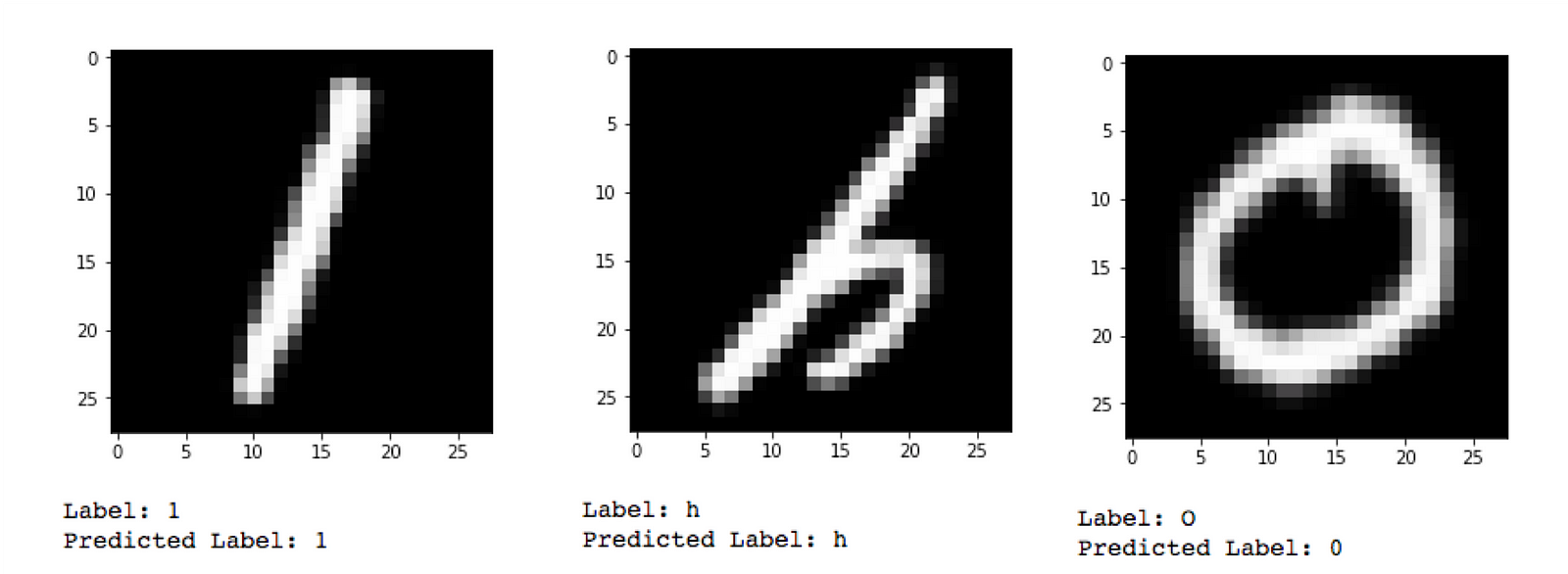
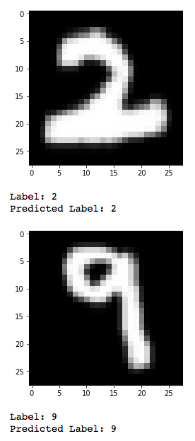
We end up with an accuracy of 78.3% on our 1000 test examples which is consistent compared to our training results. Finally let’s have a look at some examples below. We can spot that the model struggles differentiating a capitalized O from 0 which is not easy at all.

Model Deployment: Flask Webservice

In this section, we will turn to our final deployment approach. Therefore, we embed model inference within a simple webservice and build a minimalist frontend that allows the user to upload images for classification. For this purpose, we use Flask, which is a neat web development framework for Python and based on Werkzeug and Jinja2. We will implement the module emnist_dl2prod.emnist_webserver in the package itself, but you can refer to this JuPyter notebook for additional information.

There are three parts for this section:

1. Build Model Wrapper Class
2. Implement the Webservice and Frontend
3. Run and Test our own EMNIST Webserver

1. Build Model Wrapper Class

We start with the model wrapper class below. In order to create a new instance, we have to provide the path to the model that was previously saved using the SavedModelBuilder. Here, we use the loader functionality of tf.saved_model to load and restore our model. We also create a session in which we restore the graph definition and variables that constitute our SavedModel. The model class furthermore implements a run method to easily perform single instance or batch-wise inference later on. This method simply runs the session on flattened and normalized image data (float values between 0 and 1) and returns the softmax activation across all 62 classes.

2. Implement the Webservice and Frontend

Next, we turn to Flask and some HTML as we combine the simple REST webservice with a minimalist frontend to upload images and to visualize the classification result. First, we create two HTML files, img_upload.html and result.html. The first page implements an image upload interface and a button to submit the image data which internally triggers the preprocessing and classification process. The latter file resembles a template to display the uploaded image itself and of course to show the classification result. The result is the detected (most probable) class as well as the softmax scores our model comes up with. Let’s have a closer look to what happens in between. Upon image upload, the upload page triggers the following redirect: url_for('process_img_upload'). This redirect provides the following method with a POST-request:

emnist_result is a dictionary we use to finally render our results’ page with proper values. This also requires to temporarily save the uploaded image and check for the correct filetype. In the latter part, we read the image using skimage which directly yields a NumPy array — data scientists’ darling. Afterwards, we preprocess (normalization + flatten) and classify the image array simply invoking run of our model wrapper instance as part of classify_img. This returns the softmax activation values and maps the index of the highest activation to a proper label. In the end, we complete our request result by adding softmax values and label to the dictionary and call show_emnist_result that renders the results’ page.

Besides our frontend showcase, we also implement a method that answers a POST-request with a proper response object instead of rendering any HTML templates:

3. Testing and Peformance Evaluation

Once again, it’s time to reap the fruits of our labor. We start our webserver and let process some examples. You can either start it using python emnist_webserver.py or use the command emnist-webservice that was installed with the package. Either way, you should something similar to the following in your terminal:

[2018-10-14 11:07:26] INFO:__main__:Set up temporary media folder for webserver: /Users/mkurovski/Python/emnist_dl2prod/src/emnist_dl2prod/tmp_flask_media * Serving Flask app "emnist_webserver" (lazy loading) * Environment: production   WARNING: Do not use the development server in a production environment.   Use a production WSGI server instead. * Debug mode: off[2018-10-14 11:07:26] INFO:werkzeug: * Running on http://0.0.0.0:5000/ (Press CTRL+C to quit)

Great! Let’s pay it a visit:

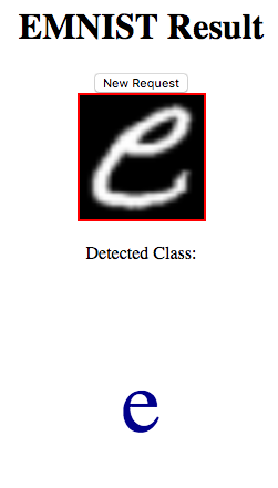
In order to easily test this, you can find the folder test_images in the repository that contains 10 characters. Try out a few! We choose an image and click Get Result and `voilà` we see e and a 99.74% probability among the softmax activations. On the backend side we receive further confirmation that everything went as expected:

[14/Oct/2018 11:11:26] "POST /emnist/result HTTP/1.1" 200 -[14/Oct/2018 11:11:26] "GET /emnist/img_upload/img_upload_1539508286216.png HTTP/1.1" 200 -

In the related JuPyter notebook, you will see some examples for our latter implementation that we also want to try out here. For evaluation and testing purposes, you can find eval_serving_performance as part of emnist_dl2prod.utils. This method creates a certain amount of requests from test or train data, sends them to a specified endpoint and evaluates the accuracy of responses as well as their times. We will cover it in more detail in the next part. Here, let’s just try it out on the endpoint we just created:

This visualizes some of the results and tells us the average accuracy for our requests:

Accuracy on 1000 test images: 77.60%

77.6% — Yeah! That looks pretty consistent with our training experience.Great! We implemented our own webservice which successfully confirmed our training results in production. It is time for the finals — how do all these approaches compare with each other in a qualitative and quantitative sense?

Conclusion: Comparing Throughput and Prediction Accuracy across Different Deployments

This is the final part of my comprehensive blogpost series on deep learning model exploration, translation, and production. With a multitude of technologies like Docker, TensorFlow, GraphPipe, PyTorch, ONNX and Flask we build approaches that bridge the gap from exploration to production. All approaches started off with PyTorch for exploration and ONNX for translation. They differ in the way we deployed each solution. We started with GraphPipe and Docker to provide a short and simple wrapper that processes REST calls. We continued using TensorFlow Serving itself within a Docker container. This was a little more verbose and complicated. Finally, we used Flask to build our own webserver and embed model inference calls. We also combined the last approach with a minimalist frontend. This was the most verbose, but also the most understandable way for deployment. However, I wouldn’t recommend using it for large-scale production systems, it is helpful to capture how model inference, client-server communication and frontend are connected with each other. Now, let’s have a look at how these approaches compare with each other in qualitative and quantitative terms.

First, let’s have a qualitative look in terms of ease of use and implementation effort. In my view, Flask is the easiest way to go — with GraphPipe close behind it. Some unexpected failures in GraphPipe serving ONNX models caused trouble. However, shifting to TensorFlow easily resolved our issue back then. With TensorFlow Serving things can become a little complicated and therefore it takes the third place for this aspect. Regarding the extent our implementations took, GraphPipe is the clear winner with very few code to deploy our models. TensorFlow Serving needs a little more, but still does quite OK. The definition of signatures adds some verbosity here. Flask is close behind, as it takes significantly more effort as GraphPipe which seems self-evident for building own solutions.

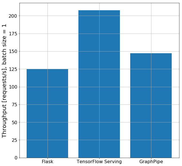
But, as data scientists and engineers we are more interested in numbers as a mere gut feeling. Therefore, I was also interested in how these deployments compare given the request throughput and if they return consistent results. Refer to this JuPyter notebook for the comparison. I tested all solutions on a Google Cloud compute instance with a single CPU. However, to avoid measurements biased by poor internet connection, I am showing results for locally hosting each service here. We cover to scenarios: sending single instance requests and batch requests with 128 exampled each. For both scenarios, we use a single client thread and no asynchronous requests to stay consistent with how Oracle’s evaluated GraphPipe. We then count the number of successful requests within a consistent duration and obtain the throughputs per second as performance metric. See emnist_dl2prod.utils:eval_throughput for the implementation of our throughput test. It’s important to note that the absolute numbers may vary across different settings. However this shouldn’t be our concern here, as we are rather interested in how these approaches compare with each other instead of their individual absolute performance. So, let’s take a look at the single instance request throughput. We clearly see TensorFlow Serving outperforming GraphPipe and Flask serving over 200 single instance requests per second where GraphPipe and Flask excel approximately 150, respectively 125.

Differences become far stronger if we look into the batch inference case using and the order has changed. GraphPipe clearly stands out serving approximately three times more images as TensorFlow Serving does in the same time. TensorFlow Serving scores second best processing approximately 70–80% more requests as the Flask webservice does.

This is quite consistent with Oracle’s claim. However magnitudes don’t turn out to be as extreme in our case.

In conclusion, GraphPipe is significantly faster as Flask and TensorFlow when it comes to batch inference. However, TensorFlow Serving clearly excels for single instance inference which is important to note. In case we don’t batch incoming requests and provide GraphPipe with them, we better stay with TensorFlow Serving. But, if our problem allows for it or if we can batch incoming requests, we better go for GraphPipe.

Outlook

Wow, that was a lot and I hope you still enjoyed it. Please try it out yourself, share your experience and let’s try to mind the gap between exploration and production. There is a multitude of technologies supporting us and even more to come. In particular, I expect ONNX to become even more an integral part of deep learning frameworks and GraphPipe to advance beyond its current status. With these and other contributions we can bring things far more easier into production and make AI serve the people by transforming their lifes.