
決策樹分類鳶尾花資料demo
阿新 • • 發佈:2019-01-07
code:
import numpy as np
import pandas as pd
import matplotlib.pyplot as plt
import matplotlib as mpl
from sklearn import tree
from sklearn.tree import DecisionTreeClassifier
from sklearn.model_selection import train_test_split
from sklearn.preprocessing import StandardScaler
from sklearn.pipeline import Pipeline
import pydotplus

if __name__ == "__main__":

	iris_feature_E = "sepal lenght", "sepal width", "petal length", "petal width"
	iris_feature = "the length of sepal", "the width of sepal", "the length of petal", "the width of petal"
	iris_class = "Iris-setosa", "Iris-versicolor", "Iris-virginica"

	data = pd.read_csv("iris.data", header=None)
	iris_types = data[4].unique()
	for i, type in enumerate(iris_types):
		data.set_value(data[4] == type, 4, i)
	x, y = np.split(data.values, (4,), axis=1)
	x_train, x_test, y_train, y_test = train_test_split(x, y, train_size=0.7, random_state=1)
	print(y_test)

	model = DecisionTreeClassifier(criterion='entropy', max_depth=6)
	model = model.fit(x_train, y_train)
	y_test_hat = model.predict(x_test)
	with open('iris.dot', 'w') as f:
		tree.export_graphviz(model, out_file=f)
	dot_data = tree.export_graphviz(model, out_file=None, feature_names=iris_feature_E, class_names=iris_class,
		filled=True, rounded=True, special_characters=True)
	graph = pydotplus.graph_from_dot_data(dot_data)
	graph.write_pdf('iris.pdf')
	f = open('iris.png', 'wb')
	f.write(graph.create_png())
	f.close()

	# 畫圖
	# 橫縱各取樣多少個值
	N, M = 50, 50
	# 第0列的範圍
	x1_min, x1_max = x[:, 0].min(), x[:, 0].max()
	# 第1列的範圍
	x2_min, x2_max = x[:, 1].min(), x[:, 1].max()
	t1 = np.linspace(x1_min, x1_max, N)
	t2 = np.linspace(x2_min, x2_max, M)
	# 生成網格取樣點
	x1, x2 = np.meshgrid(t1, t2)
    # # 無意義,只是為了湊另外兩個維度
    # # 開啟該註釋前,確保註釋掉x = x[:, :2]
	x3 = np.ones(x1.size) * np.average(x[:, 2])
	x4 = np.ones(x1.size) * np.average(x[:, 3])
	# 測試點
	x_show = np.stack((x1.flat, x2.flat, x3, x4), axis=1)
	print("x_show_shape:\n", x_show.shape)

	cm_light = mpl.colors.ListedColormap(['#77E0A0', '#FF8080', '#A0A0FF'])
	cm_dark = mpl.colors.ListedColormap(['g', 'r', 'b'])
	# 預測值
	y_show_hat = model.predict(x_show)
	print(y_show_hat.shape)
	print(y_show_hat)
	# 使之與輸入的形狀相同
	y_show_hat = y_show_hat.reshape(x1.shape)
	print(y_show_hat)
	plt.figure(figsize=(15, 15), facecolor='w')
	# 預測值的顯示
	plt.pcolormesh(x1, x2, y_show_hat, cmap=cm_light)
	print(y_test)
	print(y_test.ravel())
	# 測試資料
	plt.scatter(x_test[:, 0], x_test[:, 1], c=np.squeeze(y_test), edgecolors='k', s=120, cmap=cm_dark, marker='*')
	# 全部資料
	plt.scatter(x[:, 0], x[:, 1], c=np.squeeze(y), edgecolors='k', s=40, cmap=cm_dark)
	plt.xlabel(iris_feature[0], fontsize=15)
	plt.ylabel(iris_feature[1], fontsize=15)
	plt.xlim(x1_min, x1_max)
	plt.ylim(x2_min, x2_max)
	plt.grid(True)
	plt.title('yuanwei flowers regressiong with DecisionTree', fontsize=17)
	plt.show()

	# 訓練集上的預測結果
	y_test = y_test.reshape(-1)
	print(y_test_hat)
	print(y_test)
	# True則預測正確,False則預測錯誤
	result = (y_test_hat == y_test)
	acc = np.mean(result)
	print('accuracy: %.2f%%' % (100 * acc))

    # 過擬合:錯誤率
	depth = np.arange(1, 15)
	err_list = []
	for d in depth:
		clf = DecisionTreeClassifier(criterion='entropy', max_depth=d)
		clf = clf.fit(x_train, y_train)
		# 測試資料
		y_test_hat = clf.predict(x_test)
		# True則預測正確,False則預測錯誤
		result = (y_test_hat == y_test)
		err = 1 - np.mean(result)
		err_list.append(err)
		print(d, 'error ratio: %.2f%%' % (100 * err))
	plt.figure(figsize=(15, 15), facecolor='w')
	plt.plot(depth, err_list, 'ro-', lw=2)
	plt.xlabel('DecisionTree Depth', fontsize=15)
	plt.ylabel('error ratio', fontsize=15)
	plt.title('DecisionTree Depth and Overfit', fontsize=17)
	plt.grid(True)
plt.show() 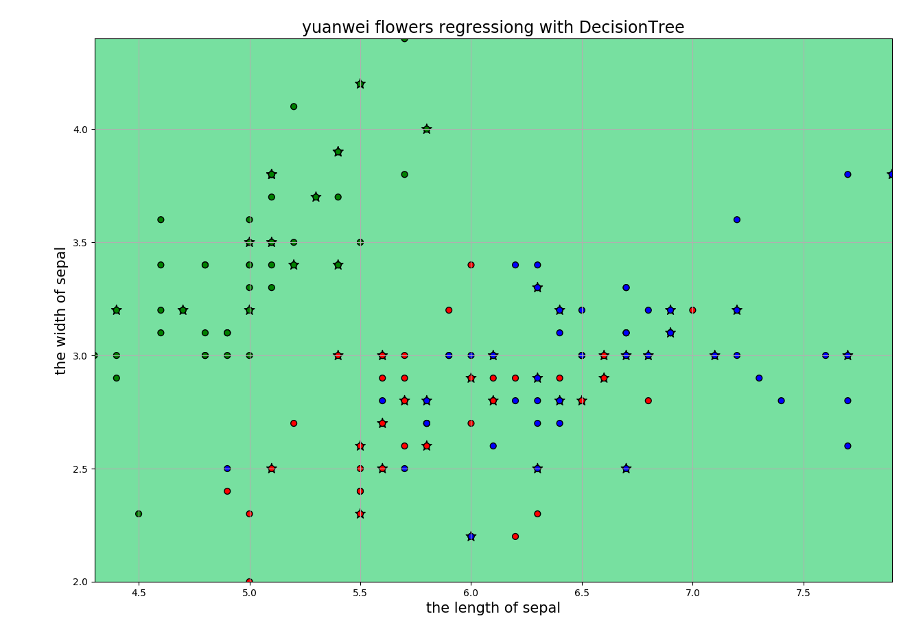


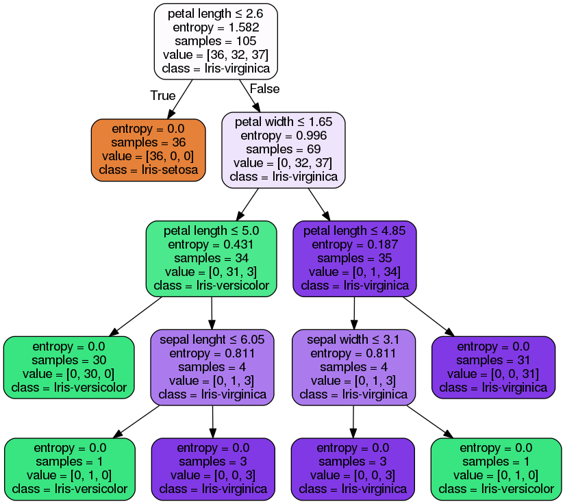
生成的圖檔案:
鳶尾花的資料特徵一共有四種:花萼長度、花萼寬度,花瓣長度,花瓣寬度。然後再使用決策樹兩兩特徵進行分類:
import numpy as np
import pandas as pd
import matplotlib.pyplot as plt
import matplotlib as mpl
from sklearn import tree
from sklearn.tree import DecisionTreeClassifier
from sklearn.model_selection import train_test_split
from sklearn.preprocessing import StandardScaler
from sklearn.pipeline import Pipeline
import pydotplus
if __name__ == "__main__":
iris_feature_E = "sepal lenght", "sepal width", "petal length", "petal width"
iris_feature = "the length of sepal", "the width of sepal", "the length of petal", "the width of petal"
iris_class = "Iris-setosa", "Iris-versicolor", "Iris-virginica"
data = pd.read_csv("iris.data", header=None)
iris_types = data[4].unique()
for i, type in enumerate(iris_types):
data.set_value(data[4] == type, 4, i)
x_train, y = np.split(data.values, (4,), axis=1)
feature_pairs = [(0, 1), (0, 2), (0, 3), (1, 2), (1, 3), (2, 3)]
plt.figure(figsize=(15, 15), facecolor='w')
for i, pair in enumerate(feature_pairs):
# 準備資料
x = x_train[:, pair]
# 決策樹進行學習
clf = DecisionTreeClassifier(criterion='entropy', min_samples_leaf=3)
dt_clf = clf.fit(x, y)
# 開始畫圖
N, M = 500, 500
# 第0列的範圍
x1_min, x1_max = x[:, 0].min(), x[:, 0].max()
# 第1列的範圍
x2_min, x2_max = x[:, 1].min(), x[:, 1].max()
t1 = np.linspace(x1_min, x1_max, N)
t2 = np.linspace(x2_min, x2_max, M)
# 生成網格取樣點
x1, x2 = np.meshgrid(t1, t2)
# 測試點
x_test = np.stack((x1.flat, x2.flat), axis=1)
# 在訓練集上預測結果
y_hat = dt_clf.predict(x)
y = y.reshape(-1)
# 統計預測正確的個數
c = np.count_nonzero(y_hat == y)
print("y_hat:\n", y_hat)
print("y:\n", y)
'''
set1 = set(y_hat)
set2 = set(y)
print(list(set1 & set2))
if y_hat.any() != y.any():
print('predict:%.3f real:%.3f' %(y_hat.all(), y.all()))
'''
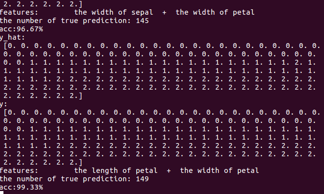
# 列印相關資訊
print('features:\t', iris_feature[pair[0]], ' + ', iris_feature[pair[1]])
print('the number of true prediction:', c)
print('acc:%.2f%%' %(100 * float(c) / float(len(y))))
# 畫圖顯示
cm_light = mpl.colors.ListedColormap(['#77E0A0', '#FF8080', '#A0A0FF'])
cm_dark = mpl.colors.ListedColormap(['g', 'r', 'b'])
# 預測值
y_test_hat = dt_clf.predict(x_test)
# reshape到和輸入的x1相同格式
y_test_hat = y_test_hat.reshape(x1.shape)
plt.subplot(2, 3, i+1)
plt.pcolormesh(x1, x2, y_test_hat, cmap=cm_light)
plt.scatter(x[:, 0], x[:, 1], c=y, edgecolors='k', cmap=cm_dark)
plt.xlabel(iris_feature[pair[0]], fontsize=14)
plt.ylabel(iris_feature[pair[1]], fontsize=14)
plt.xlim(x1_min, x1_max)
plt.ylim(x2_min, x2_max)
plt.grid()
plt.suptitle('the result of yuanwei flowers in each two features with dcisiontree', fontsize=20)
plt.tight_layout(2)
plt.subplots_adjust(top=0.92)
plt.show() 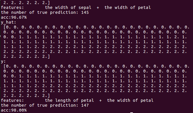
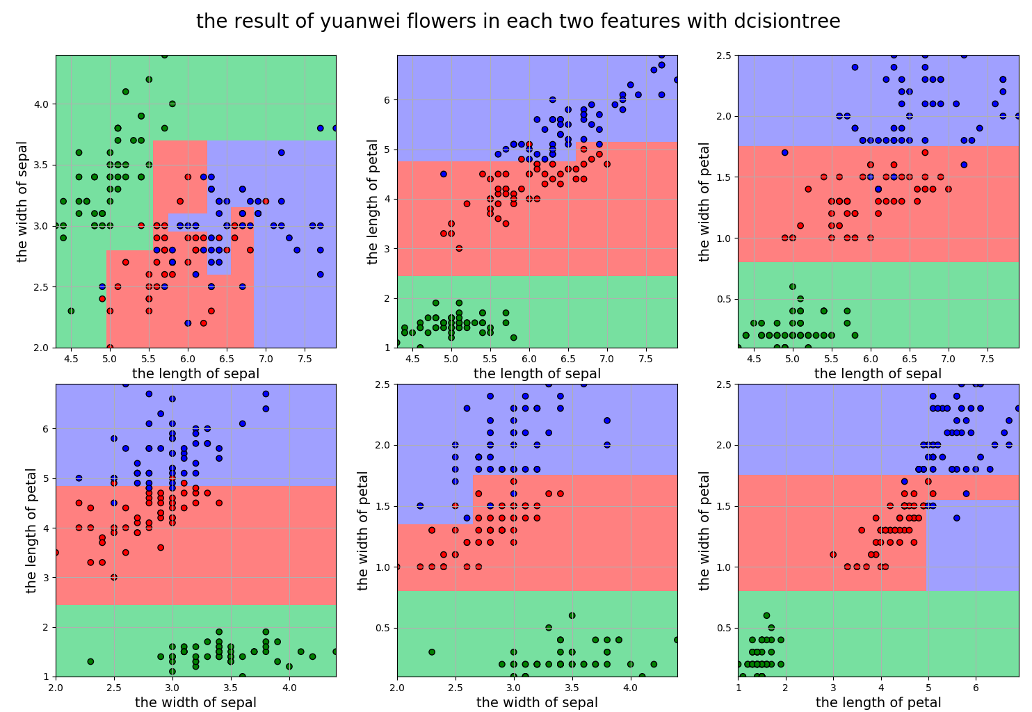
顯然第二種組合效果還可以的。
接著我們使用隨機森林演算法來分類看看效果:
只需要在上面的程式碼中修改:
# 決策樹進行學習
clf = DecisionTreeRegressor(n_estimators=200, criterion='entropy', max_depth=6)
為:
# 決策樹進行學習
clf = RandomForestClassifier(n_estimators=200, criterion='entropy', max_depth=6)
效果:
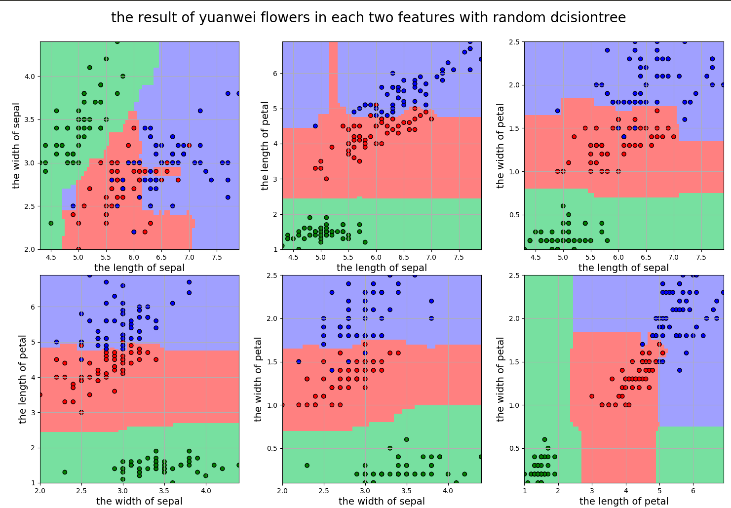
看得出來隨機森林的分類要比決策樹好,隨機森林因為是根據多個決策樹弱分類器聯合成一個強分類器,所以其邊界出呈現很多的鋸齒,分類的準確度也提高很多,150個數據,最後只有一個分錯。