
deeplearning.ai課程作業:Course 1 Week 2
deeplearning.ai課程作業:Course 1 Week 2
原始作業在GitHub上下載,本文僅作為本人學習過程的記錄,含答案,不喜勿看。全部自己跑過,保證可行。
Part 1:Python Basics with Numpy (optional assignment)
Welcome to your first assignment. This exercise gives you a brief introduction to Python. Even if you’ve used Python before, this will help familiarize you with functions we’ll need.
Instructions:
- You will be using Python 3.
- Avoid using for-loops and while-loops, unless you are explicitly told to do so.
- Do not modify the (# GRADED FUNCTION [function name]) comment in some cells. Your work would not be graded if you change this. Each cell containing that comment should only contain one function.
- After coding your function, run the cell right below it to check if your result is correct.
After this assignment you will:
- Be able to use iPython Notebooks
- Be able to use numpy functions and numpy matrix/vector operations
- Understand the concept of “broadcasting”
- Be able to vectorize code
Let’s get started!
About iPython Notebooks
iPython Notebooks are interactive coding environments embedded in a webpage. You will be using iPython notebooks in this class. You only need to write code between the ### START CODE HERE ### and ### END CODE HERE ### comments. After writing your code, you can run the cell by either pressing “SHIFT”+”ENTER” or by clicking on “Run Cell” (denoted by a play symbol) in the upper bar of the notebook.
We will often specify “(≈ X lines of code)” in the comments to tell you about how much code you need to write. It is just a rough estimate, so don’t feel bad if your code is longer or shorter.
Exercise: Set test to “Hello World” in the cell below to print “Hello World” and run the two cells below.
### START CODE HERE ### (≈ 1 line of code)
test = "Hello World"
### END CODE HERE ###
print ("test: " + test)
test: Hello World
Expected output:
test: Hello World
What you need to remember:
- Run your cells using SHIFT+ENTER (or “Run cell”)
- Write code in the designated areas using Python 3 only
- Do not modify the code outside of the designated areas
1 - Building basic functions with numpy
Numpy is the main package for scientific computing in Python. It is maintained by a large community (www.numpy.org). In this exercise you will learn several key numpy functions such as np.exp, np.log, and np.reshape. You will need to know how to use these functions for future assignments.
1.1 - sigmoid function, np.exp()
Exercise: Build a function that returns the sigmoid of a real number x. Use math.exp(x) for the exponential function.
Reminder:
sigmoid(x)=11+e−xsigmoid(x)=11+e−x is sometimes also known as the logistic function. It is a non-linear function used not only in Machine Learning (Logistic Regression), but also in Deep Learning.
To refer to a function belonging to a specific package you could call it using package_name.function(). Run the code below to see an example with math.exp().
# GRADED FUNCTION: basic_sigmoid

import math

def basic_sigmoid(x):
    """
    Compute sigmoid of x.

    Arguments:
    x -- A scalar

    Return:
    s -- sigmoid(x)
    """

    ### START CODE HERE ### (≈ 1 line of code)
    s = 1 / (1 + 1/ math.exp(x))
    ### END CODE HERE ###

    return s
basic_sigmoid(3)
0.9525741268224334
Expected Output:
| Input | Output |
|---|---|
| basic_sigmoid(3) | 0.9525741268224334 |
Actually, we rarely use the “math” library in deep learning because the inputs of the functions are real numbers. In deep learning we mostly use matrices and vectors. This is why numpy is more useful.
### One reason why we use "numpy" instead of "math" in Deep Learning ###
x = [1, 2, 3]
basic_sigmoid(x) # you will see this give an error when you run it, because x is a vector.
---------------------------------------------------------------------------

TypeError                                 Traceback (most recent call last)

<ipython-input-3-2e11097d6860> in <module>()
      1 ### One reason why we use "numpy" instead of "math" in Deep Learning ###
      2 x = [1, 2, 3]
----> 3 basic_sigmoid(x) # you will see this give an error when you run it, because x is a vector.


<ipython-input-1-65a96864f65f> in basic_sigmoid(x)
     15
     16     ### START CODE HERE ### (≈ 1 line of code)
---> 17     s = 1.0 / (1 + 1/ math.exp(x))
     18     ### END CODE HERE ###
     19


TypeError: a float is required
In fact, if is a row vector then np.exp(x)np.exp(x) will apply the exponential function to every element of x. The output will thus be:
import numpy as np

# example of np.exp
x = np.array([1, 2, 3])
print(np.exp(x)) # result is (exp(1), exp(2), exp(3))
[ 2.71828183 7.3890561 20.08553692]
Furthermore, if x is a vector, then a Python operation such as or will output s as a vector of the same size as x.
# example of vector operation
x = np.array([1, 2, 3])
print (x + 3)
[4 5 6]
Any time you need more info on a numpy function, we encourage you to look at the official documentation.
You can also create a new cell in the notebook and write np.exp? (for example) to get quick access to the documentation.
Exercise: Implement the sigmoid function using numpy.
Instructions: x could now be either a real number, a vector, or a matrix. The data structures we use in numpy to represent these shapes (vectors, matrices…) are called numpy arrays. You don’t need to know more for now.
# GRADED FUNCTION: sigmoid

import numpy as np # this means you can access numpy functions by writing np.function() instead of numpy.function()

def sigmoid(x):
    """
    Compute the sigmoid of x

    Arguments:
    x -- A scalar or numpy array of any size

    Return:
    s -- sigmoid(x)
    """

    ### START CODE HERE ### (≈ 1 line of code)
    s = 1.0 / (1 + 1 / np.exp(x))
    ### END CODE HERE ###

    return s
x = np.array([1, 2, 3])
sigmoid(x)
array([ 0.73105858, 0.88079708, 0.95257413])
1.2 - Sigmoid gradient
Exercise: Implement the function sigmoid_grad() to compute the gradient of the sigmoid function with respect to its input x. The formula is:
You often code this function in two steps:
1.Set s to be the sigmoid of x. You might find your sigmoid(x) function useful.
2.Compute
# GRADED FUNCTION: sigmoid_derivative

def sigmoid_derivative(x):
    """
    Compute the gradient (also called the slope or derivative) of the sigmoid function with respect to its input x.
    You can store the output of the sigmoid function into variables and then use it to calculate the gradient.

    Arguments:
    x -- A scalar or numpy array

    Return:
    ds -- Your computed gradient.
    """

    ### START CODE HERE ### (≈ 2 lines of code)
    s = 1.0 / (1 + 1 / np.exp(x))
    ds = s * (1 - s)
    ### END CODE HERE ###

    return ds
x = np.array([1, 2, 3])
print ("sigmoid_derivative(x) = " + str(sigmoid_derivative(x)))
sigmoid_derivative(x) = [ 0.19661193 0.10499359 0.04517666]
1.3 - Reshaping arrays
Two common numpy functions used in deep learning are np.shape and np.reshape().
- X.shape is used to get the shape (dimension) of a matrix/vector X.
- X.reshape(…) is used to reshape X into some other dimension.
For example, in computer science, an image is represented by a 3D array of shape
. However, when you read an image as the input of an algorithm you convert it to a vector of shape
. In other words, you “unroll”, or reshape, the 3D array into a 1D vector.
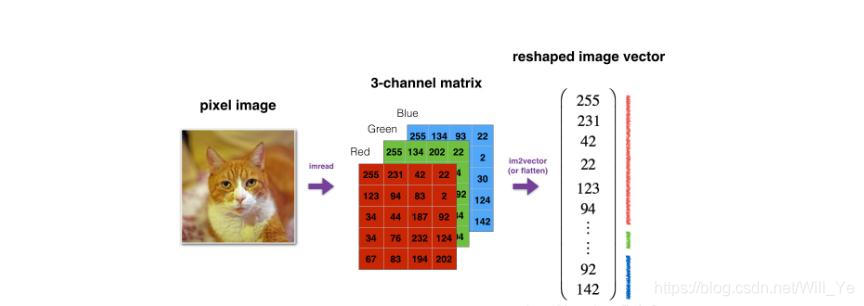
Exercise: Implement image2vector() that takes an input of shape (length, height, 3) and returns a vector of shape (lengthheight3, 1). For example, if you would like to reshape an array v of shape (a, b, c) into a vector of shape (a*b,c) you would do:
v = v.reshape((v.shape[0]*v.shape[1], v.shape[2])) # v.shape[0] = a ; v.shape[1] = b ; v.shape[2] = c
- Please don’t hardcode the dimensions of image as a constant. Instead look up the quantities you need with image.shape[0], etc.
# GRADED FUNCTION: image2vector
def image2vector(image):
    """
    Argument:
    image -- a numpy array of shape (length, height, depth)

    Returns:
    v -- a vector of shape (length*height*depth, 1)
    """

    ### START CODE HERE ### (≈ 1 line of code)
    v = image.reshape((image.shape[0] * image.shape[1] * image.shape[2], 1))
    ### END CODE HERE ###

    return v
# This is a 3 by 3 by 2 array, typically images will be (num_px_x, num_px_y,3) where 3 represents the RGB values
image = np.array([[[ 0.67826139,  0.29380381],
        [ 0.90714982,  0.52835647],
        [ 0.4215251 ,  0.45017551]],

       [[ 0.92814219,  0.96677647],
        [ 0.85304703,  0.52351845],
        [ 0.19981397,  0.27417313]],

       [[ 0.60659855,  0.00533165],
        [ 0.10820313,  0.49978937],
        [ 0.34144279,  0.94630077]]])

print ("image2vector(image) = " + str(image2vector(image)))
image2vector(image) = [[ 0.67826139]
 [ 0.29380381]
 [ 0.90714982]
 [ 0.52835647]
 [ 0.4215251 ]
 [ 0.45017551]
 [ 0.92814219]
 [ 0.96677647]
 [ 0.85304703]
 [ 0.52351845]
 [ 0.19981397]
 [ 0.27417313]
 [ 0.60659855]
 [ 0.00533165]
 [ 0.10820313]
 [ 0.49978937]
 [ 0.34144279]
 [ 0.94630077]]
1.4 - Normalizing rows
Another common technique we use in Machine Learning and Deep Learning is to normalize our data. It often leads to a better performance because gradient descent converges faster after normalization. Here, by normalization we mean changing x to (dividing each row vector of x by its norm).
For example,if