電影評論好壞分類(隨筆)

載入資料集

from keras.datasets import imdb
(train_data, train_labels),(test_data,test_labels) = imdb.load_data(num_words=10000)
##此處10000是為了保留訓練資料中前10000個最常出現的單詞，並拋棄低頻的單詞，保證資料不會太大

解碼評論,將整數轉換成單詞

## 將單詞對映為以整數為索引的字典
word_index = imdb.get_word_index()
## 鍵值顛倒，將索引轉為單詞
reverse_word_index = dict([(value,key) for (key,value) in word_index.items()])
## 解碼函式
def decode_review(text):
    return ' '.join([reverse_word_index.get(i-3, '?') for i in text])
 

樣例

decode_review(trian_data[0])

"? this film was just brilliant casting location scenery story direction everyone's really suited the part they played and you could just imagine being there robert ? is an amazing actor and now the same being director ? father came from the same scottish island as myself so i loved the fact there was a real connection with this film the witty remarks throughout the film were great it was just brilliant so much that i bought the film as soon as it was released for ? and would recommend it to everyone to watch and the fly fishing was amazing really cried at the end it was so sad and you know what they say if you cry at a film it must have been good and this definitely was also ? to the two little boy's that played the ? of norman and paul they were just brilliant children are often left out of the ? list i think because the stars that play them all grown up are such a big profile for the whole film but these children are amazing and should be praised for what they have done don't you think the whole story was so lovely because it was true and was someone's life after all that was shared with us all"

顯而易見train_data[0]是個好評

train_labels[0]
output: 1

不過這只是個開始，還要考慮每個評論長短不一的問題，因為神經網路的輸入要求長度相同,所以在此需要處理一下資料

準備資料

先把列表轉換成張量

1. 填充列表
2. 用one-hot編碼，將整個列表轉為0和1的向量，比如序列[3,5]，在轉為10000維的向量的時候，只有索引3,5下才是1，其他是0

以下是one-hot的程式碼，跟著書本上來的

import numpy as np
def vectorize_sequence(sequence,dimension=10000):
    results = np.zeros((len(sequence),dimension)) ## 建立一個形狀為(len(sequence),dimension)的零矩陣
    for i,sq in enumerate(sequence):
        results[i,sq] = 1.
    return results
x_train = vectorize_sequence(train_data)
x_test = vectorize_sequence(test_data)
## 將labels向量化
y_train =np.asarray(train_labels).astype('float32')
y_test = np.asarray(test_labels).astype('float32')
 

構建網路

先用Keras構建一個3層的神經網路

from keras import models
from keras import layers
model = models.Sequential()
## 構建輸入層，設定16個輸入單元,並設定10000維的輸入張量,啟用函式就relu吧
model.add(layers.Dense(16,activation='relu',input_shape=(10000,)))
## 隱藏層，設定16個隱藏單元，同樣activation為relu
model.add(layers.Dense(16,activation='relu'))
## 輸出層,僅包含一個單元，因為就是輸出判斷好評與否，因為要控制在0-1之間所以啟用函式是sigmoid
model.add(layers.Dense(1,activation='sigmoid'))

驗證方法

在此我們設定一個驗證集，之前聽說過訓練集以及測試集，在這裡驗證集就是一個衡量的標準吧

x_val = x_train[:10000]
partial_x_train=x_train[10000:]
y_val = y_train[:10000]
partial_y_train = y_train[10000:]

訓練模型

from keras import losses
from keras import metrics
from keras import optimizers
## 編譯模型,優化器選擇rmsprop,損失函式選擇二叉熵
model.compile(optimizer = 'rmsprop',
             loss = 'binary_crossentropy',
             metrics=['accuracy'])


history = model.fit(partial_x_train,
                    partial_y_train,
                    epochs=20,
                    batch_size=512,
                    ## 驗證資料傳入validation_data來完成
                    validation_data=(x_val,y_val))

繪製訓練損失和驗證損失

import matplotlib.pyplot as plt
history_dict=history.history
loss_values = history_dict['loss']
val_loss_values = history_dict['val_loss']
epochs = range(1,len(loss_values)+1)
plt.plot(epochs,loss_values,'bo',label='Training loss')
plt.plot(epochs,val_loss_values,'b',label='Validation loss')
plt.title('Training and validation loss')
plt.xlabel('Epochs')
plt.ylabel('Loss')
plt.legend()
plt.show()

如下圖所示:

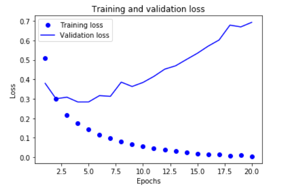
圖中，圓點是Train loss，折線是Validation loss，可見週期越大，訓練的損失越小，但驗證損失卻在大約第四輪之後變大了，這就是overfit了，因此我們這裡只用4次的epoch就可以達到最優了

從頭訓練一個模型

這裡我們讓epochs=4

model = models.Sequential()
model.add(layers.Dense(16,activation='relu',input_shape=(10000,)))
model.add(layers.Dense(16,activation='relu'))
model.add(layers.Dense(1,activation='sigmoid'))
model.compile(optimizer='rmsprop',
             loss ='binary_crossentropy',
             metrics=['accuracy'])
model.fit(x_train,y_train,epochs=4,batch_size=512)
results = model.evaluate(x_test,y_test)

得到的結果是:

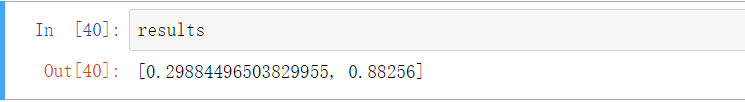
這裡的精度是88%左右並可以用以下程式碼檢視評論是否正面

model.predict(x_test)

看《Pythons深度學習》之後，給自己做的一個筆記
其中也借鑑了下
https://blog.csdn.net/qq_20084101/article/details/82054749