
利用線性迴歸模型進行kaggle房價預測
最近剛學線性迴歸的一些基礎知識,就想利用kaggle中的一個入門級比賽 House Prices: Advanced Regression Techniques進行一下鞏固,發現建模之前的資料清洗與特徵選擇非常重要。
1. 資料清洗
1.1 匯入資料
將train.csv與test.csv檔案匯入,放到一起直接預處理,處理完畢後再分開。
def load_file(path):    #匯入資料
    f = open(path)
    train_set = pd.read_csv(f, index_col=0)
    return train_set

train_path = "G:\practice.pycharm\house_price_predict\\train.csv"
train_set = load_file(train_path)
test_path = "G:\practice.pycharm\house_price_predict\\all\\test.csv"
all_set = pd.concat([train_set,load_file(train_path)])
可以利用shape函式得到train與all的大小,便於處理後分割
print(train_set.shape)
(1460, 80)
print(all_set.shape)
(2919, 80)
1.2 資料預處理
1.2.1 資料去重
使用drop_duplicates函式去掉重複值:
DataFrame.drop_duplicates(subset=None, keep='first', inplace=False)這裡因為我們需要對所有列進行重複行刪除,保留第一個值即可,這裡直接使用預設引數。
all_set.drop_duplicates(keep='first',inplace=True)
shape檢視發現沒有重複值:
(2919, 80)1.2.2 缺失值處理
na_count = all_set.shape[0]-all_set.count().sort_values()
na_rate = na_count/all_set.shape[0]
na_det = pd.concat([na_count,na_rate],axis=1,keys=['nan count','nan ratio'])
print(na_det.head(36))
nan count nan ratio PoolQC 2909 0.996574 MiscFeature 2814 0.964029 Alley 2721 0.932169 Fence 2348 0.804385 SalePrice 1459 0.499829 FireplaceQu 1420 0.486468 LotFrontage 486 0.166495 GarageYrBlt 159 0.054471 GarageFinish 159 0.054471 GarageCond 159 0.054471 GarageQual 159 0.054471 GarageType 157 0.053786 BsmtCond 82 0.028092 BsmtExposure 82 0.028092 BsmtQual 81 0.027749 BsmtFinType2 80 0.027407 BsmtFinType1 79 0.027064 MasVnrType 24 0.008222 MasVnrArea 23 0.007879 MSZoning 4 0.001370 Utilities 2 0.000685 BsmtFullBath 2 0.000685 BsmtHalfBath 2 0.000685 Functional 2 0.000685 SaleType 1 0.000343 KitchenQual 1 0.000343 TotalBsmtSF 1 0.000343 BsmtFinSF1 1 0.000343 Electrical 1 0.000343 GarageCars 1 0.000343 GarageArea 1 0.000343 BsmtFinSF2 1 0.000343 Exterior2nd 1 0.000343 Exterior1st 1 0.000343 BsmtUnfSF 1 0.000343 RoofMatl 0 0.000000
一共發現有35個包含缺失值的列,一般的,當一列資料缺失值超過15%時,就應該刪除該列,注意到SalePrice列為我們要預測的列,所有除SalePice外其餘6列全部予以刪除。
all_set.drop('PoolQC',axis = 1,inplace = True)
all_set.drop('MiscFeature', axis=1, inplace=True)
all_set.drop('Alley', axis=1, inplace=True)
all_set.drop('Fence', axis=1, inplace=True)
all_set.drop('FireplaceQu', axis=1, inplace=True)
all_set.drop('LotFrontage', axis=1, inplace=True)
而後面GarageX的項,應該是一些列強相關的項,因為有GarageCars這個特徵表徵,也可以刪去。
all_set.drop('GarageYrBlt', axis=1, inplace=True)
all_set.drop('GarageFinish', axis=1, inplace=True)
all_set.drop('GarageCond', axis=1, inplace=True)
all_set.drop('GarageQual', axis=1, inplace=True)
all_set.drop('GarageType', axis=1, inplace=True)
對於BsmtX同樣刪除。
all_set.drop('BsmtCond', axis=1, inplace=True)
all_set.drop('BsmtExposure', axis=1, inplace=True)
all_set.drop('BsmtQual', axis=1, inplace=True)
all_set.drop('BsmtFinType2', axis=1, inplace=True)
all_set.drop('BsmtFinType1', axis=1, inplace=True)
對於MasVnr也同樣刪除。
all_set.drop('MasVnrType', axis=1, inplace=True)
all_set.drop('MasVnrArea', axis=1, inplace=True)
檢視另外18列含有缺失值的屬性。
              nan count  nan ratio    dtype
SalePrice          1459   0.499829  float64
MSZoning              4   0.001370   object
Utilities             2   0.000685   object
BsmtFullBath          2   0.000685  float64
BsmtHalfBath          2   0.000685  float64
Functional            2   0.000685   object
Exterior1st           1   0.000343   object
GarageCars            1   0.000343  float64
Exterior2nd           1   0.000343   object
SaleType              1   0.000343   object
Electrical            1   0.000343   object
GarageArea            1   0.000343  float64
BsmtUnfSF             1   0.000343  float64
BsmtFinSF2            1   0.000343  float64
BsmtFinSF1            1   0.000343  float64
TotalBsmtSF           1   0.000343  float64
KitchenQual           1   0.000343   object
Neighborhood          0   0.000000   object
發現這些列中有的是object屬性,有的是float屬性,分別進行處理,對於object屬性的列,使用出現頻率最高的值進行代替,對於float屬性的列,一般為“無”,所以不填,故使用0填充。
all_set['MSZoning'].fillna('C (all)',inplace=True)
all_set['Utilities'].fillna('AllPub',inplace=True)
all_set['Functional'].fillna('Typ',inplace=True)
all_set['Exterior1st'].fillna('VinylSd',inplace=True)
all_set['Exterior2nd'].fillna('VinylSd',inplace=True)
all_set['SaleType'].fillna('WD',inplace=True)
all_set['Electrical'].fillna('SBrkr',inplace=True)
all_set['KitchenQual'].fillna('TA',inplace=True)
all_set['BsmtFullBath'].fillna(0., inplace=True)
all_set['BsmtHalfBath'].fillna(0., inplace=True)
all_set['BsmtUnfSF'].fillna(0., inplace=True)
all_set['GarageArea'].fillna(0., inplace=True)
all_set['GarageCars'].fillna(0., inplace=True)
all_set['TotalBsmtSF'].fillna(0., inplace=True)
all_set['BsmtFinSF1'].fillna(0., inplace=True)
all_set['BsmtFinSF2'].fillna(0., inplace=True)再次對缺失值進行檢查,發現除我們要預測的SalePrice列外沒有缺失值,缺失值處理完畢。
              nan count  nan ratio    dtype
SalePrice          1459   0.499829  float64
1stFlrSF              0   0.000000    int64
LandSlope             0   0.000000   object
LotArea               0   0.000000    int64
LotConfig             0   0.000000   object
LotShape              0   0.000000   object
LowQualFinSF          0   0.000000    int64
MSSubClass            0   0.000000    int64
MSZoning              0   0.000000   object
MiscVal               0   0.000000    int64
1.2.3 定性量啞編碼
對資料集進行onehot啞編碼,將定性量轉化為啞編碼方式,便於後續訓練模型,將原資料集中的SalePrice列刪除。
data_set.drop('SalePrice',axis = 1,inplace = True)
data_set_num = pd.DataFrame()
data_set_ob = pd.DataFrame()
for i in data_set.columns.values:
    if data_set[i].dtypes == 'object':
        data_set_ob = pd.concat([data_set_ob,data_set[i]],axis=1)
    else:
        data_set_num = pd.concat([data_set_num,data_set[i]],axis=1)
data_set_ob = pd.get_dummies(data_set)
得到啞編碼後的資料集,檢視shape:
(2918, 221)1.2.4 連續值標準化
為提高收斂速度,對資料集標準化,對價格取對數。選擇sklearn中的StandardScaler進行標準化,價格採用log1p函式。
num_col = data_set_num.columns
data_set_num = pd.DataFrame(preprocessing.StandardScaler().fit_transform(data_set_num),columns=num_col)
data_y = np.log1p(data_y)檢視對數化之前與之後的分佈:


對數化後更加符合正態分佈。
1.2.5 離群值刪除
首先拿到所有單列對於價格的散點圖:


發現GrLivArea明顯有兩個偏離點,找到刪除。
data_x.drop(data_x.index[[1298,523]],inplace = True)
data_y.drop(data_y.index[[1298,523]],inplace = True)


離群點刪除完畢。
2. 資料建模
2.1 資料分割
將資料集按7:3切割為訓練集和測試集。
x_train,x_test,y_train,y_test = cross_validation.train_test_split(data_x,data_y,test_size=0.3)2.2 線性迴歸模型
利用sklearn中的線性模型對訓練集進行建模。
model = linear_model.LinearRegression()
model.fit(x_train,y_train)
使用多元線性迴歸擬合數據,檢視截距與係數:
係數: [-1.85543669e+07 -8.04763021e+06  8.74505546e-02 -8.41983585e-02
  2.60674291e+10  7.04799731e+09  8.07989649e-02 -2.37079067e-02
  1.07890706e+10  9.29348469e-02  1.55423164e-01  8.64651203e-02
  1.88232660e-01  1.80189371e-01  2.06861132e+07  3.56459618e-02
 -8.52451324e-02  7.75563359e-01 -4.14657567e+06 -7.68175125e-02
 -5.87408125e-01  1.83105469e-03  1.02868974e-02  4.62743044e-01
  6.69234022e-01  1.10272944e-01  1.84955835e-01  1.72290325e-01
 -2.82197009e+10  3.00650597e-02  4.03986931e-01  7.40909576e-02
 -2.11348534e-02 -2.70690585e+10 -2.70690585e+10 -2.70690585e+10
 -2.70690585e+10 -2.70690585e+10  1.53694722e+10  1.53694722e+10
  5.55073126e+08  5.55073126e+08  5.55073126e+08  5.55073126e+08
  5.55073126e+08  5.55073126e+08  5.55073126e+08  5.55073126e+08
  5.55073126e+08 -1.71070683e+10 -1.71070683e+10 -1.71070683e+10
 -2.20707567e+10 -1.71070683e+10 -1.71070683e+10 -1.71070683e+10
 -1.71070683e+10  3.77141831e+10  3.77141831e+10  3.77141831e+10
 -3.58089763e+10  3.77141831e+10  6.11169150e+09  6.11169150e+09
  6.11169150e+09  6.11169150e+09  6.11169150e+09 -6.32708343e+08
 -6.32708343e+08 -6.32708343e+08 -6.32708343e+08 -9.89338552e+09
 -9.89338552e+09 -9.89338552e+09 -9.89338552e+09 -1.68585564e+10
 -9.89338552e+09 -9.89338552e+09 -9.89338552e+09 -9.89338552e+09
 -9.89338552e+09 -9.89338552e+09 -9.89338552e+09 -9.89338552e+09
 -9.89338552e+09 -9.89338552e+09  1.43397977e+10  1.43397977e+10
  1.43397977e+10  1.43397977e+10  2.13049686e+10  1.43397977e+10
  1.43397977e+10  1.43397977e+10  1.43397977e+10  3.21889821e+10
  1.43397977e+10  1.43397977e+10  1.43397977e+10  1.43397977e+10
  1.43397977e+10  1.43397977e+10 -3.28284039e+09 -3.28284039e+09
 -3.28284039e+09 -3.28284039e+09 -3.28284039e+09 -3.28284039e+09
  1.02802487e+09  1.02802487e+09  1.02802487e+09  1.02802487e+09
  1.02802487e+09 -1.73231695e+09  1.02802487e+09  1.65177921e+09
  1.65177921e+09  1.65177921e+09  1.65177921e+09  1.65177921e+09
  1.65177921e+09 -5.89256168e+10 -5.89256168e+10 -5.89256168e+10
  2.93173824e+09 -5.89256168e+10 -2.05874740e+10 -2.05874740e+10
 -2.05874740e+10 -2.05874740e+10 -2.05874740e+10 -2.05874740e+10
 -2.05874740e+10 -2.05874740e+10 -1.88074328e+10 -1.88074328e+10
 -1.88074328e+10 -1.88074328e+10 -8.77449366e+09 -8.77449366e+09
 -8.77449366e+09 -8.77449366e+09  3.12362451e+10  3.12362451e+10
  3.12362451e+10 -6.76533101e+09 -6.76533101e+09 -6.76533101e+09
 -6.76533101e+09 -6.76533101e+09  1.74194848e+10  1.74194848e+10
  1.74194848e+10  1.74194848e+10 -2.32040189e+10 -2.32040189e+10
 -2.32040189e+10 -2.32040189e+10 -2.32040189e+10 -9.22089572e+09
 -9.22089572e+09 -9.22089572e+09 -9.22089572e+09 -9.22089572e+09
 -9.22089572e+09 -9.22089572e+09 -9.22089572e+09 -9.22089572e+09
 -9.22089572e+09 -9.22089572e+09 -9.22089572e+09 -9.22089572e+09
 -9.22089572e+09 -9.22089572e+09 -9.22089572e+09 -9.22089572e+09
 -9.22089572e+09 -9.22089572e+09 -9.22089572e+09 -9.22089572e+09
 -9.22089572e+09 -9.22089572e+09 -9.22089572e+09 -9.22089572e+09
  1.05481999e+10  1.05481999e+10  1.05481999e+10  2.45233811e+08
  2.45233811e+08  2.45233811e+08  2.45233811e+08  2.45233811e+08
  2.45233811e+08  2.45233811e+08  2.45233811e+08 -1.65389315e+08
 -1.65389315e+08 -1.65389315e+08 -1.65389315e+08 -1.65389315e+08
 -1.65389315e+08 -4.98004278e+08 -4.98004278e+08 -4.98004278e+08
 -4.98004278e+08 -4.98004278e+08 -4.98004278e+08 -1.40919590e+10
 -1.40919590e+10 -1.40919590e+10 -1.40919590e+10 -1.40919590e+10
 -1.40919590e+10 -1.40919590e+10 -1.40919590e+10 -1.40919590e+10
 -2.06193399e+09 -2.06193399e+09 -8.50851018e+08 -8.50851018e+08]
截距: 85719276156.30911
3. 模型評估
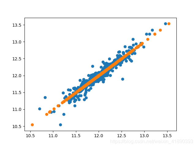
3.1 視覺化
將預測值與目標值放入一張圖進行比較。
y_pre = model.predict(x_test)plt.scatter(y_pre,y_test,marker='o')
plt.scatter(y_test,y_test)
plt.show()
擬合度看起來還行, 看一下方差的大小。
print(metrics.mean_squared_error(y_test,y_pre))
0.015132547556096164
3.2 模型調整
3.2.1 正則化引數
線上性迴歸模型中加入正則化項,使用sklearn中的Ridge建立具有正則化項的線性迴歸模型。
model = linear_model.Ridge(alpha=i)
model.fit(x_train,y_train)
畫出正則化項隨偏差的變化趨勢。

可見aplha取1是比較合理的,此時Jcv(紅色曲線)接近最低值,Jtrain值也比較低。
3.2.2 樣本分割比例
將誤差根據訓練樣本大小畫出曲線。

樣本分割比例的修改對誤差的影響不大(一般取6:2:2)。
3.2.3 迭代次數
迭代次數無需調整。
3.2.4 視覺化
將預測值與目標值重新作圖,得到:

可見效果還不錯,可以輸出提交了。
4. 總結
這是我第一次做kaggle比賽,也是從0開始,從資料清洗到建模到調整,全部按照自己的主觀想法來做,所以會比較隨意,後續也會逐漸再改進。