目錄

WLLS

LLS review

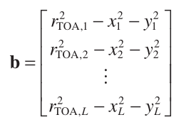
前面有博文：LLS，提到了線性最小二乘演算法，使用LLS去求解TOA-Based Positioning問題，從推導過程看起來很簡單。具體說來，關鍵就是這幾個公式：

當噪聲足夠小，q可以近似為：

這是一個零均值的向量，最後我們求得

具體推導過程，參見開頭推薦的那篇博文。

從此處看，還是很簡單的。今天的主題是WLLS，也就是加權最小二乘法，與LLS有著千絲萬縷的關係。下面娓娓道來！

WLLS

Although the LLS approach is simple, it provides optimum estimation performance only when the disturbances in the linear equations are independent and identically distributed.

儘管LLS方法很簡單，但只有當線性方程中的擾動是獨立且相同分佈時，它才能提供最佳估計效能。

From Equations 2.83 and 2.92 , it is obvious that the LLS – TOA - based positioning algorithms are suboptimal.

從方程2.83和2.92，很明顯基於LLS - TOA的定位演算法是次優的。

Taking Equation 2.85 as an illustration, the localization accuracy can be improved if we include a symmetric weighting matrix, say, W

, in the cost function, denoted by .

 The resultant expression is referred to as the WLS cost function, which has the form of

注：式子2.85如下，為LLS演算法的代價函式：

According to Equations 2.82 and 2.83 , we have E { b } = A θ , which corresponds to the linear unbiased data model. As a result, we can follow the best linear unbiased estimator ( BLUE ) [19, 28] to determine the optimum W

, which is equal to the inverse of the covariance of q ; that is, the weighting matrix is similar to that of the ML methodology. Employing Equation 2.83 , we obtain

根據方程2.82和2.83，我們得到E {b} =Aθ，其對應於線性無偏資料模型。 結果，我們可以遵循最佳線性無偏估計（BLUE）[19,28]來確定最優W，它等於q的協方差的倒數; 也就是說，加權矩陣類似於ML方法的加權矩陣。 使用公式2.83，我們得到

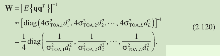
As { } are not available, a practical choice of W is to replace  with , which is valid for sufficiently small error condition:

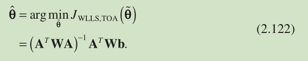
Following Equations 2.86 and 2.87 , the WLLS estimate of θ is

注：

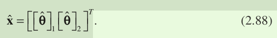
The WLLS position estimate is then given as Equation 2.88 .

the two - step WLS estimator

With only a moderate increase of computational complexity [19] , Equation 2.122 is superior to Equation 2.87 in terms of estimation performance.

Nevertheless, the localization accuracy can be further enhanced by making use of   according to the relation of Equation 2.76 as follows. When   of Equation 2.122 is sufficiently close to x , we have

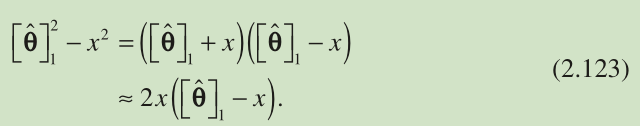
Similarly, for 

注：

Based on Equation 2.76 and with the use of Equations 2.123 and 2.124 , we construct

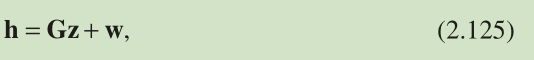
where

Note that z is the parameter vector to be determined. To find the covariance of w , we utilize the result of BLUE that the covariance of  is of the form of [28]

Employing Equations 2.129 and 2.130 , the optimal weighting matrix for Equation 2.125 , denoted by Φ , is then

As a result, the WLLS estimate of z is

As there is no sign information for x in z , the final position estimate is determined as

where sgn represents the signum function. In the literature, this approach is called the two - step WLS estimator [20] , where Equation 2.76 is exploited in an implicit manner. Alternatively, an explicit way is to minimize Equation 2.119 subject to the constraint of Equation 2.76 , which can be solved by the method of Lagrangian multipliers [21, 22] .

其中sgn代表signum函式。 在文獻中，這種方法被稱為兩步WLS估計器[20]，其中方程2.76以隱式方式被利用。 或者，一種明確的方法是在方程2.76的約束下最小化方程2.119，這可以通過拉格朗日乘數法[21,22]求解。

注：