Diving into a Practical Keras Example

Two-class classification, or binary classification, may be the most widely applied kind of machine-learning problem. In this example, you’ll learn to classify movie reviews as positive or negative, based on the text content of the reviews.

You’ll work with the IMDB dataset: a set of 50,000 highly polarized reviews from the Internet Movie Database. They’re split into 25,000 reviews for training and 25,000 reviews for testing, each set consisting of 50% negative and 50% positive reviews.

Just like the MNIST dataset, the IMDB dataset comes packaged with Keras. It has already been preprocessed: the reviews (sequences of words) have been turned into sequences of integers, where each integer stands for a specific word in a dictionary.

The following code will load the dataset (when you run it the first time, about 80 MB of data will be downloaded to your machine).

>>> from keras.datasets import imdb

>>> (train_data, train_labels), (test_data, test_labels) = imdb.load_data(num_words=10000)

The argument num_words=10000 means you’ll only keep the top 10,000 most frequently occurring words in the training data. Rare words will be discarded. This allows you to work with vector data of manageable size.

The variables train_data and test_data are lists of reviews; each review is a list of word indices (encoding a sequence of words). train_labels and test_labels are lists of 0s and 1s, where 0 stands for negative and 1 stands for positive:

>>> train_data[0][1, 14, 22, 16, ... 178, 32]

>>> train_labels[0]1

Because you’re restricting yourself to the top 10,000 most frequent words, no word index will exceed 10,000:

>>> max([max(sequence) for sequence in train_data])9999

For kicks, here’s how you can quickly decode one of these reviews back to English words:

>>> word_index = imdb.get_word_index()Downloading data from https://s3.amazonaws.com/text-datasets/imdb_word_index.json1646592/1641221 [==============================] - 1s 0us/step

>>> reverse_word_index = dict([(value, key) for (key, value) in word_index.items()])>>> decoded_review = ' '.join([reverse_word_index.get(i - 3, '?') for i in train_data[0]])

Preparing the Data

You can’t feed lists of integers into a neural network. You have to turn your lists into tensors. There are two ways to do that:

1. Pad your lists so that they all have the same length, turn them into an integer tensor of shape (samples, word_indices), and then use as the first layer in your network a layer capable of handling such integer tensors (the Embedding layer).
2. One-hot encode your lists to turn them into vectors of 0s and 1s. This would mean, for instance, turning the sequence [3, 5] into a 10,000-dimensional vector that would be all 0s except for indices 3 and 5, which would be 1s. Then you could use as the first layer in your network a Dense layer, capable of handling floating-point vector data.

Let’s go with the latter solution to vectorize the data, which you’ll do manually for maximum clarity.

>>> import numpy as np

>>> def vectorize_sequences(sequences, dimension=10000):...     results = np.zeros((len(sequences), dimension))...     for i, sequence in enumerate(sequences):...             results[i, sequence] = 1...     return results... 

>>> x_train = vectorize_sequences(train_data)>>> x_test = vectorize_sequences(test_data)

Here’s what the samples look like now:

>>> x_train[0]array([ 0.,  1.,  1., ...,  0.,  0.,  0.])

You should also vectorize your labels, which is straightforward:

>>> y_train = np.asarray(train_labels).astype('float32')

>>> y_test = np.asarray(test_labels).astype('float32')

Now the data is ready to be fed into a neural network.

Building your network

The input data is vectors, and the labels are scalars (1s and 0s): this is the easiest setup you’ll ever encounter. A type of network that performs well on such a problem is a simple stack of fully connected (Dense) layers with relu activations: Dense(16, activation=’relu’)

The argument being passed to each Dense layer (16) is the number of hidden units of the layer. A hidden unit is a dimension in the representation space of the layer. From the following equation:

output = relu(dot(W, input) + b)

Having 16 hidden units means the weight matrix W will have shape (input_dimension, 16): the dot product with W will project the input data onto a 16-dimensional representation space (and then you’ll add the bias vector b and apply the relu operation). You can intuitively understand the dimensionality of your representation space as “how much freedom you’re allowing the network to have when learning internal representations.” Having more hidden units (a higher-dimensional representation space) allows your network to learn more-complex representations, but it makes the network more computationally expensive and may lead to learning unwanted patterns (patterns that will improve performance on the training data but not on the test data).

There are two key architecture decisions to be made about such a stack of Dense layers:

1. How many layers to use?
2. How many hidden units to choose for each layer?

We’ll go with the following:

1. Two intermediate layers with 16 hidden units each
2. A third layer that will output the scalar prediction regarding the sentiment of the current review

The intermediate layers will use relu as their activation function, and the final layer will use a sigmoid activation so as to output a probability (a score between 0 and 1, indicating how likely the sample is to have the target “1”: how likely the review is to be positive).

A relu (rectified linear unit) is a function meant to zero out negative values:

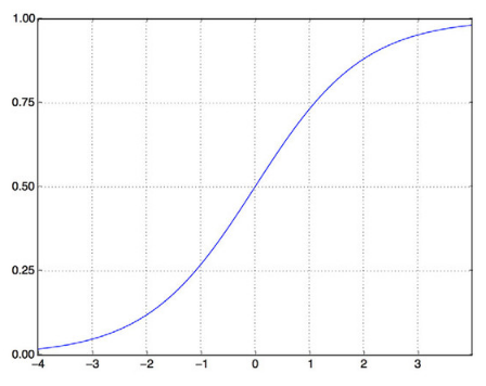
Whereas a sigmoid “squashes” arbitrary values into the [0, 1] interval, outputting something that can be interpreted as a probability:

This is what the network looks like from a high-level:

And here’s the Keras implementation, similar to the MNIST example you saw previously.

>>> from keras import models>>> from keras import layers

>>> model = models.Sequential()>>> model.add(layers.Dense(16, activation='relu', input_shape=(10000,)))>>> model.add(layers.Dense(16, activation='relu'))>>> model.add(layers.Dense(1, activation='sigmoid'))

Finally, you need to choose a loss function and an optimizer. Because you’re facing a binary classification problem and the output of your network is a probability (you end your network with a single-unit layer with a sigmoid activation), it’s best to use the binary_crossentropy loss. It isn’t the only viable choice: you could use, for instance, mean_squared_error. But crossentropy is usually the best choice when you’re dealing with models that output probabilities. Crossentropy is a quantity from the field of Information Theory that measures the distance between probability distributions or, in this case, between the ground-truth distribution and your predictions.

Here’s the step where you configure the model with the rmsprop optimizer and the binary_crossentropy loss function. Note that you’ll also monitor accuracy during training.

>>> model.compile(optimizer='rmsprop', loss='binary_crossentropy', metrics=['accuracy'])

You’re passing your optimizer, loss function, and metrics as strings, which is possible because rmsprop, binary_crossentropy, and accuracy are packaged as part of Keras. Sometimes you may want to configure the parameters of your optimizer or pass a custom loss function or metric function. The former can be done by passing an optimizer class instance as the optimizer argument:

>>> from keras import optimizers

>>> model.compile(optimizer=optimizers.RMSprop(lr=0.001), loss='binary_crossentropy', metrics=['accuracy'])

The latter can be done by passing function objects as the lossand/or metrics arguments:

>>> from keras import losses>>> from keras import metrics>>> model.compile(optimizer=optimizers.RMSprop(lr=0.001), loss=losses.binary_crossentropy, metrics=[metrics.binary_accuracy])

Validating Your Approach

In order to monitor during training the accuracy of the model on data it has never seen before, you’ll create a validation set by setting apart 10,000 samples from the original training data.

>>> x_val = x_train[:10000]>>> partial_x_train = x_train[10000:]>>> y_val = y_train[:10000]>>> partial_y_train = y_train[10000:]

You’ll now train the model for 20 epochs (20 iterations over all samples in the x_train and y_train tensors), in mini-batches of 512 samples. At the same time, you’ll monitor loss and accuracy on the 10,000 samples that you set apart. You do so by passing the validation data as the validation_data argument.

>>> model.compile(optimizer='rmsprop', loss='binary_crossentropy', metrics=['acc'])

>>> history = model.fit(partial_x_train, partial_y_train, epochs=20, batch_size=512, validation_data=(x_val, y_val))Train on 15000 samples, validate on 10000 samplesEpoch 1/202018-08-31 12:21:39.007625: I tensorflow/core/platform/cpu_feature_guard.cc:141] Your CPU supports instructions that this TensorFlow binary was not compiled to use: AVX2 FMA15000/15000 [==============================] - 3s 176us/step - loss: 0.5084 - acc: 0.7813 - val_loss: 0.3797 - val_acc: 0.8684Epoch 2/2015000/15000 [==============================] - 2s 114us/step - loss: 0.3004 - acc: 0.9047 - val_loss: 0.3004 - val_acc: 0.8897Epoch 3/2015000/15000 [==============================] - 2s 113us/step - loss: 0.2179 - acc: 0.9285 - val_loss: 0.3085 - val_acc: 0.8711Epoch 4/2015000/15000 [==============================] - 2s 114us/step - loss: 0.1750 - acc: 0.9437 - val_loss: 0.2840 - val_acc: 0.8832Epoch 5/2015000/15000 [==============================] - 2s 113us/step - loss: 0.1427 - acc: 0.9543 - val_loss: 0.2841 - val_acc: 0.8872Epoch 6/2015000/15000 [==============================] - 2s 114us/step - loss: 0.1150 - acc: 0.9650 - val_loss: 0.3165 - val_acc: 0.8772Epoch 7/2015000/15000 [==============================] - 2s 113us/step - loss: 0.0980 - acc: 0.9705 - val_loss: 0.3127 - val_acc: 0.8845Epoch 8/2015000/15000 [==============================] - 2s 113us/step - loss: 0.0807 - acc: 0.9763 - val_loss: 0.3859 - val_acc: 0.8649Epoch 9/2015000/15000 [==============================] - 2s 115us/step - loss: 0.0661 - acc: 0.9821 - val_loss: 0.3635 - val_acc: 0.8782Epoch 10/2015000/15000 [==============================] - 2s 119us/step - loss: 0.0561 - acc: 0.9853 - val_loss: 0.3843 - val_acc: 0.8792Epoch 11/2015000/15000 [==============================] - 2s 118us/step - loss: 0.0440 - acc: 0.9893 - val_loss: 0.4153 - val_acc: 0.8778Epoch 12/2015000/15000 [==============================] - 2s 115us/step - loss: 0.0382 - acc: 0.9919 - val_loss: 0.4524 - val_acc: 0.8690Epoch 13/2015000/15000 [==============================] - 2s 115us/step - loss: 0.0300 - acc: 0.9928 - val_loss: 0.4698 - val_acc: 0.8728Epoch 14/2015000/15000 [==============================] - 2s 115us/step - loss: 0.0247 - acc: 0.9946 - val_loss: 0.5023 - val_acc: 0.8730Epoch 15/2015000/15000 [==============================] - 2s 115us/step - loss: 0.0175 - acc: 0.9980 - val_loss: 0.5347 - val_acc: 0.8695Epoch 16/2015000/15000 [==============================] - 2s 114us/step - loss: 0.0150 - acc: 0.9979 - val_loss: 0.5709 - val_acc: 0.8699Epoch 17/2015000/15000 [==============================] - 2s 115us/step - loss: 0.0147 - acc: 0.9969 - val_loss: 0.6024 - val_acc: 0.8692Epoch 18/2015000/15000 [==============================] - 2s 115us/step - loss: 0.0085 - acc: 0.9993 - val_loss: 0.6854 - val_acc: 0.8628Epoch 19/2015000/15000 [==============================] - 2s 113us/step - loss: 0.0062 - acc: 0.9997 - val_loss: 0.7195 - val_acc: 0.8582Epoch 20/2015000/15000 [==============================] - 2s 115us/step - loss: 0.0110 - acc: 0.9973 - val_loss: 0.6993 - val_acc: 0.8659

On a CPU, this will take less than a few seconds per epoch — training is over in 20 seconds. At the end of every epoch, there is a slight pause as the model computes its loss and accuracy on the 10,000 samples of the validation data.

Note that the call to model.fit() returns a History object. This object has a member history, which is a dictionary containing data about everything that happened during training. Let’s look at it:

>>> history_dict = history.history>>> history_dict.keys()dict_keys(['val_loss', 'loss', 'val_acc', 'acc'])

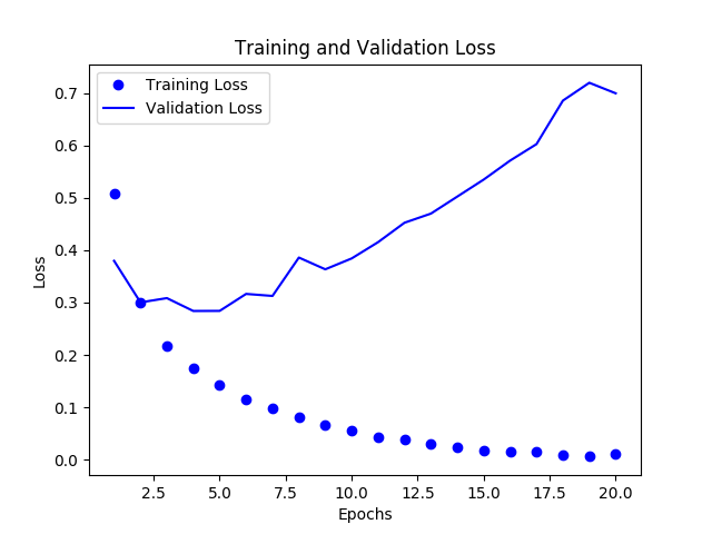
The dictionary contains four entries: one per metric that was being monitored during training and during validation. In the following two listing, let’s use Matplotlib to plot the training and validation loss side by side.

Plotting the training and validation loss:

>>> import matplotlib.pyplot as plt>>> history_dict = history.history>>> loss_values = history_dict['loss']>>> val_loss_values = history_dict['val_loss']>>> acc = history_dict['acc']>>> val_acc = history_dict['val_acc']

>>> epochs = range(1, len(acc) + 1)

>>> plt.plot(epochs, loss_values, 'bo', label='Training Loss')>>> plt.plot(epochs, val_loss_values, 'b', label='Validation Loss')>>> plt.title('Training and Validation Loss')>>> plt.xlabel('Epochs')>>> plt.ylabel('Loss')>>> plt.legend()>>> plt.show()

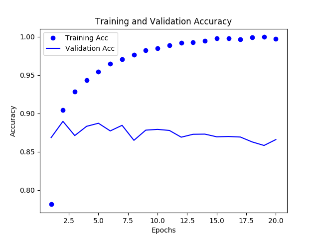
Plotting the training and validation accuracy

>>> plt.clf()>>> plt.plot(epochs, acc, 'bo', label='Training Acc')>>> plt.plot(epochs, val_acc, 'b', label='Validation Acc')>>> plt.title('Training and Validation Accuracy')>>> plt.xlabel('Epochs')>>> plt.ylabel('Accuracy')>>> plt.legend()>>> plt.show()

Note: Your own results may vary slightly due to a different random initialization of your network.

As you can see, the training loss decreases with every epoch, and the training accuracy increases with every epoch. That’s what you would expect when running gradient-descent optimization — the quantity you’re trying to minimize should be less with every iteration. But that isn’t the case for the validation loss and accuracy: they seem to peak at the fourth epoch. This is an example of what we warned against earlier: a model that performs better on the training data isn’t necessarily a model that will do better on data it has never seen before. In precise terms, what you’re seeing is overfitting: after the second epoch, you’re over-optimizing on the training data, and you end up learning representations that are specific to the training data and don’t generalize to data outside of the training set.

In this case, to prevent overfitting, you could stop training after three epochs. In general, you can use a range of techniques to mitigate overfitting.

Let’s train a new network from scratch for four epochs and then evaluate it on the test data.

>>> model = models.Sequential()>>> model.add(layers.Dense(16, activation='relu', input_shape=(10000,)))>>> model.add(layers.Dense(16, activation='relu'))>>> model.add(layers.Dense(1, activation='sigmoid'))>>> model.compile(optimizer='rmsprop', loss='binary_crossentropy', metrics=['accuracy'])>>> model.fit(x_train, y_train, epochs=4, batch_size=512)Epoch 1/425000/25000 [==============================] - 2s 88us/step - loss: 0.4749 - acc: 0.8217Epoch 2/425000/25000 [==============================] - 2s 83us/step - loss: 0.2658 - acc: 0.9097Epoch 3/425000/25000 [==============================] - 2s 81us/step - loss: 0.1982 - acc: 0.9299Epoch 4/425000/25000 [==============================] - 2s 79us/step - loss: 0.1679 - acc: 0.9404<keras.callbacks.History object at 0x7f20f00456a0>

>>> results = model.evaluate(x_test, y_test)25000/25000 [==============================] - 2s 88us/step

The final results are as follows:

>>> results[0.3231498848247528, 0.87352]

This fairly naive approach achieves an accuracy of 88%. With state-of-the-art approaches, you should be able to get close to 95%.

Using a trained network to generate predictions on new data

After having trained a network, you’ll want to use it in a practical setting. You can generate the likelihood of reviews being positive by using the predict method:

>>> model.predict(x_test)array([[0.14028223],       [0.9997029 ],       [0.29558158],       ...,       [0.07234909],       [0.04342629],       [0.48159957]], dtype=float32)

As you can see, the network is confident for some samples (0.99 or more, or 0.01 or less) but less confident for others (0.29, 0.48).

The following experiments will help convince you that the architecture choices you’ve made, of using two hidden layers, are all fairly reasonable, although there’s still room for improvement:

• Try using one or three hidden layers, and see how doing so affects validation and test accuracy.
• Try using layers with more hidden units or fewer hidden units: 32 units, 64 units, and so on.
• Try using the mse loss function instead of binary_crossentropy.
• Try using the tanh activation (an activation that was popular in the early days of neural networks) instead of relu.

Here’s what you should take away from this example:

• You usually need to do quite a bit of preprocessing on your raw data in order to be able to feed it — as tensors — into a neural network. Sequences of words can be encoded as binary vectors, but there are other encoding options, too.
• Stacks of Dense layers with relu activations can solve a wide range of problems (including sentiment classification), and you’ll likely use them frequently.
• In a binary classification problem (two output classes), your network should end with a Dense layer with one unit and a sigmoid activation: the output of your network should be a scalar between 0 and 1, encoding a probability.
• With such a scalar sigmoid output on a binary classification problem, the loss function you should use is binary_crossentropy.
• The rmsprop optimizer is generally a good enough choice, whatever your problem. That’s one less thing for you to worry about.
• As they get better on their training data, neural networks eventually start overfitting and end up obtaining increasingly worse results on data they’ve never seen before. Be sure to always monitor performance on data that is outside of the training set.