ElasticNet 是一種使用L1和L2先驗作為正則化矩陣的線性迴歸模型.這種組合用於只有很少的權重非零的稀疏模型，比如:class:Lasso, 但是又能保持:class:Ridge 的正則化屬性.我們可以使用 l1_ratio 引數來調節L1和L2的凸組合(一類特殊的線性組合)。
　　當多個特徵和另一個特徵相關的時候彈性網路非常有用。Lasso 傾向於隨機選擇其中一個，而彈性網路更傾向於選擇兩個.
　　在實踐中，Lasso 和 Ridge 之間權衡的一個優勢是它允許在迴圈過程（Under rotate）中繼承 Ridge 的穩定性.
　　
彈性網路的目標函式是最小化：

mi

ElasticNetCV 可以通過交叉驗證來用來設定引數:
alpha (α)，l1_ratio (ρ)

程式碼部分如下：

import numpy as np
from sklearn import linear_model
import warnings

warnings.filterwarnings('ignore')

###############################################################################  
 

# Generate sample data  
n_samples_train, n_samples_test, n_features = 75, 150, 500
np.random.seed(0)
coef = np.random.randn(n_features)
coef[50:] = 0.0  # only the top 10 features are impacting the model  
X = np.random.randn(n_samples_train + n_samples_test, n_features)
y = np.dot(X, coef)

# Split train and test data  
 

X_train, X_test = X[:n_samples_train], X[n_samples_train:]
y_train, y_test = y[:n_samples_train], y[n_samples_train:]

###############################################################################  
# Compute train and test errors  
alphas = np.logspace(-5, 1, 60)
enet = linear_model.ElasticNet(l1_ratio=0.7)
train_errors = list()
test_errors = list()
for alpha in alphas:
    enet.set_params(alpha=alpha)
    enet.fit(X_train, y_train)
    train_errors.append(enet.score(X_train, y_train))
    test_errors.append(enet.score(X_test, y_test))

i_alpha_optim = np.argmax(test_errors)
alpha_optim = alphas[i_alpha_optim]
print("Optimal regularization parameter : %s" % alpha_optim)

# Estimate the coef_ on full data with optimal regularization parameter  
enet.set_params(alpha=alpha_optim)
coef_ = enet.fit(X, y).coef_

###############################################################################  
# Plot results functions  

import matplotlib.pyplot as plt

plt.subplot(2, 1, 1)
plt.semilogx(alphas, train_errors, label='Train')
plt.semilogx(alphas, test_errors, label='Test')
plt.vlines(alpha_optim, plt.ylim()[0], np.max(test_errors), color='k',
           linewidth=3, label='Optimum on test')
plt.legend(loc='lower left')
plt.ylim([0, 1.2])
plt.xlabel('Regularization parameter')
plt.ylabel('Performance')

# Show estimated coef_ vs true coef  
plt.subplot(2, 1, 2)
plt.plot(coef, label='True coef')
plt.plot(coef_, label='Estimated coef')
plt.legend()
plt.subplots_adjust(0.09, 0.04, 0.94, 0.94, 0.26, 0.26)
plt.show()  

結果如下圖所示：

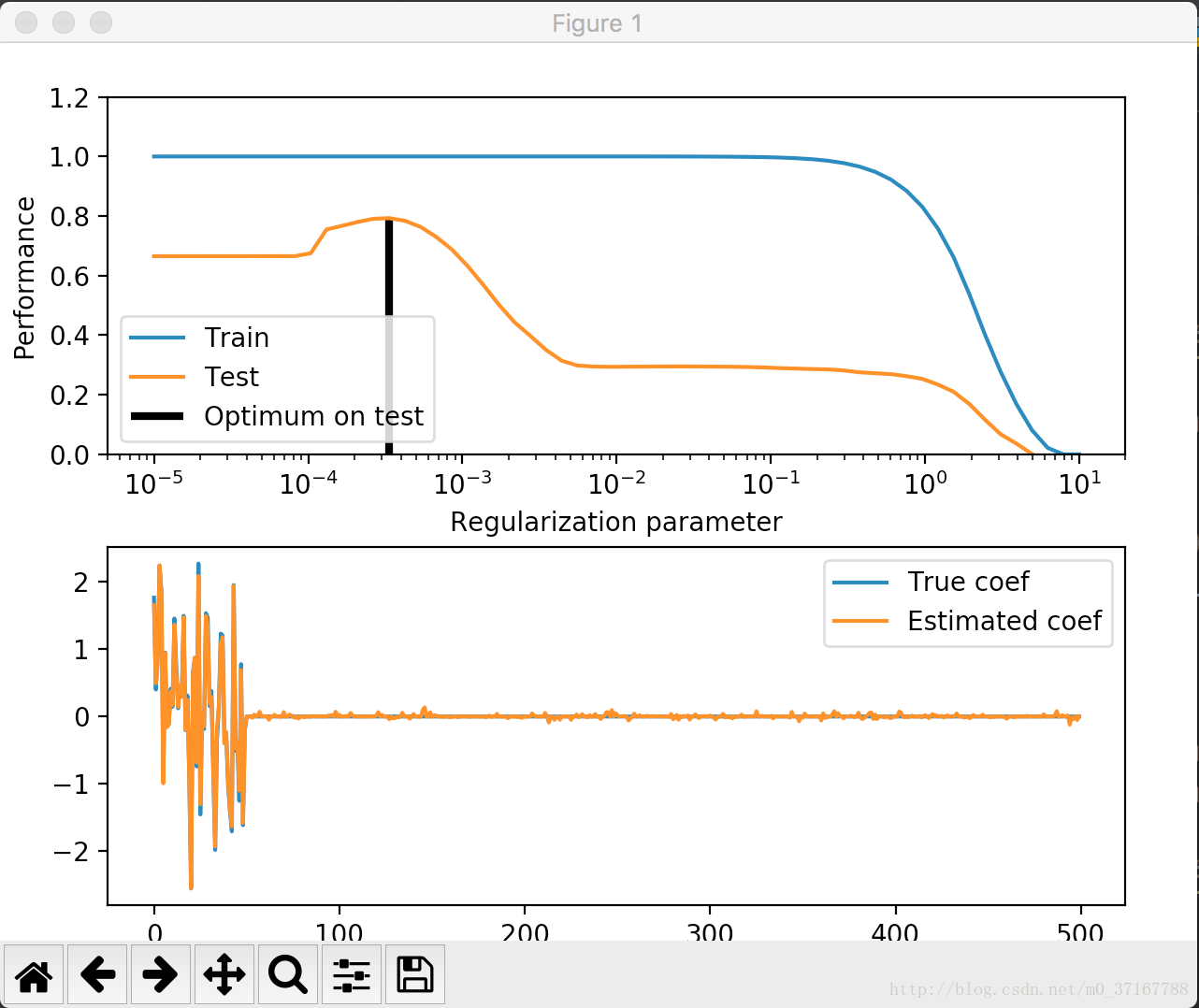
控制檯結果如下：

elastic net的大部分函式也會與之前的大體相似，所以這裡僅僅介紹一些比較經常用的到的或者特殊的引數或函式：

引數：
l1_ratio:在0到1之間，代表在l1懲罰和l2懲罰之間，如果l1_ratio=1，則為lasso，是調節模型效能的一個重要指標。
eps:Length of the path. eps=1e-3 means that alpha_min / alpha_max = 1e-3
n_alphas:正則項alpha的個數
alphas：alpha值的列表

返回值：
alphas：返回模型中的alphas值。
coefs：返回模型係數。shape=（n_feature,n_alphas）

函式：
score（X,y,sample_weight）:
評價模型效能的標準，值越接近1，模型效果越好。