機器學習筆記 多項式迴歸
上一篇機器學習筆記裡,我們講了線性迴歸.線性迴歸有一個前提:即我們假設資料是存線上性關係的. 然而,理想很豐滿,現實很骨感,現實世界裡的真實資料往往是非線性的.
比如你的資料分佈,是符合y=0.5$x^2$ + x + 2的.
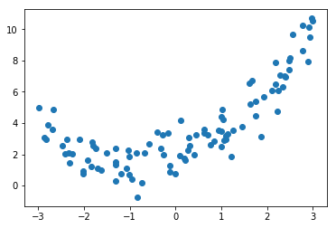
那你用y=ax+b去擬合,無論如何都沒法取的很好的效果.
這時候,我們又想繼續用上一篇筆記描述的線性迴歸來解決這個問題,我們要怎麼辦呢?一個很直觀的想法就是,我們想造出一個新的特徵$x^2$。那麼現在我們擁有了2個特徵x,$x^2$,我們就可以把問題轉換為求解y=a$x^2$ + bx +c,從而把問題轉換成我們熟悉的線性迴歸問題.
通過上面的分析,我們可以看出,我們想做的事情是對樣本做升維(即增加樣本的特徵數目),sklean中完成這一功能的類叫做
class
sklearn.preprocessing.PolynomialFeatures(degree=2, interaction_only=False, include_bias=True)degree : integer
The degree of the polynomial features. Default = 2.
interaction_only : boolean, default = False
If true, only interaction features are produced: features that are products of at most
degreedistinct input features (so notx[1] ** 2,x[0] * x[2] ** 3, etc.).include_bias : boolean
If True (default), then include a bias column, the feature in which all polynomial powers are zero (i.e. a column of ones - acts as an intercept term in a linear model).
假設你的樣本,原本有兩個特徵[a,b],那麼當你進行一次degree=2的升維之後,你將得到5個特徵[1,a,b,$a^2$,ab,$b^2$],其中1又可以看做是$a^0或者b^0$。
關於degree的理解你可以參考一下下面這個例子.from sklearn.preprocessing import PolynomialFeatures
x=pd.DataFrame({'col1': [2], 'col2': [3],'col3':[4]})
print(x)
poly2 = PolynomialFeatures(degree=2)
poly2.fit_transform(x)

>>> array([[ 1.,  2.,  3.,  4.,  4.,  6.,  8.,  9., 12., 16.]])

poly3 = PolynomialFeatures(degree=3)
poly3.fit_transform(x)

>>> array([[ 1.,  2.,  3.,  4.,  4.,  6.,  8.,  9., 12., 16.,  8., 12., 16.,
        18., 24., 32., 27., 36., 48., 64.]])
poly4 = PolynomialFeatures(degree=3,interaction_only=True)
poly4.fit_transform(x)
>>> array([[ 1., 2., 3., 4., 6., 8., 12., 24.]])
我們的樣本有3個特徵,值分別為2,3,4,degree=2時,可能的取值有$2^0$,$3^0$,$4^0$(均為1),$2^1,2^2,3^1,3^2,4^1,4^2$,$2*3,2*4,3*4$共10個值.
degree為3時,又新增了$2^3,3^3,4^3$,$2^2*3,2^2*4,3^2*2,3^2*4,4^2*2,4^2*3,2*3*4$共10個.總計20個.
interaction_only=true時,表示新增的特徵存在互動性,不存在自己*自己,比如[2,3,4]的互動式輸出是[2*3,2*4,3*4,2*3*4].
從上面的分析可以看出來,隨著degree的增加,PolynomialFeatures新生成的特徵數目是呈指數級別增加的.這將帶來模型訓練速度的嚴重下降和模型的過擬合,所以實際上一般很少用多項式迴歸.
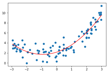
來個具體的例子
import numpy as np
import matplotlib.pyplot as plt
from sklearn.preprocessing import PolynomialFeatures

x = np.random.uniform(-3, 3, size=100)
X = x.reshape(-1, 1)
y = 0.5 * x**2 + x + 2 + np.random.normal(0, 1, 100)

#升維,為樣本生成新的特徵
poly = PolynomialFeatures(degree=2)
poly.fit(X)
X2 = poly.transform(X)

#對新樣本做訓練
from sklearn.linear_model import LinearRegression
lin_reg2 = LinearRegression()
lin_reg2.fit(X2, y)
y_predict2 = lin_reg2.predict(X2)

plt.scatter(x, y)
plt.plot(np.sort(x), y_predict2[np.argsort(x)], color='r')
plt.show()