
機器學習演算法及程式碼實現--支援向量機
阿新 • • 發佈:2019-01-09
機器學習演算法及程式碼實現–支援向量機
1、支援向量機
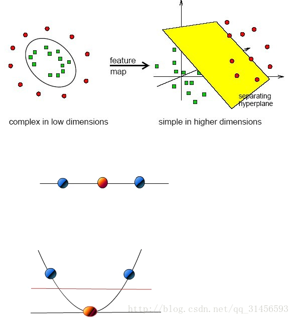
SVM希望通過N-1維的分隔超平面線性分開N維的資料,距離分隔超平面最近的點被叫做支援向量,我們利用SMO(SVM實現方法之一)最大化支援向量到分隔面的距離,這樣當新樣本點進來時,其被分類正確的概率也就更大。我們計算樣本點到分隔超平面的函式間隔,如果函式間隔為正,則分類正確,函式間隔為負,則分類錯誤,函式間隔的絕對值除以||w||就是幾何間隔,幾何間隔始終為正,可以理解為樣本點到分隔超平面的幾何距離。若資料不是線性可分的,那我們引入核函式的概念,從某個特徵空間到另一個特徵空間的對映是通過核函式來實現的,我們利用核函式將資料從低維空間對映到高維空間,低維空間的非線性問題在高維空間往往會成為線性問題,再利用N-1維分割超平面對資料分類。
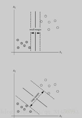
2、分類
線性可分、線性不可分
3、超平面公式(先考慮線性可分)
W*X+b=0
其中W={w1,w2,,,w3},為權重向量
下面用簡單的二維向量講解(思維導圖)
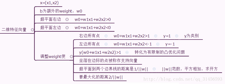
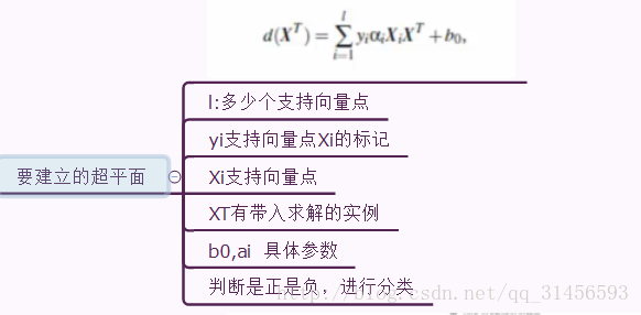
4、尋找超平面
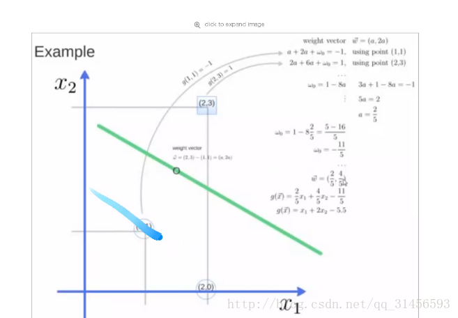
5、例子
6、線性不可分
對映到高維
演算法思路(思維導圖)
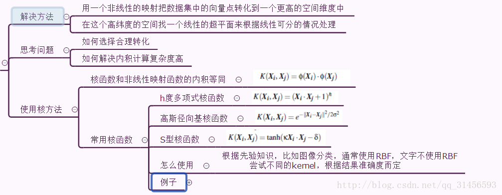
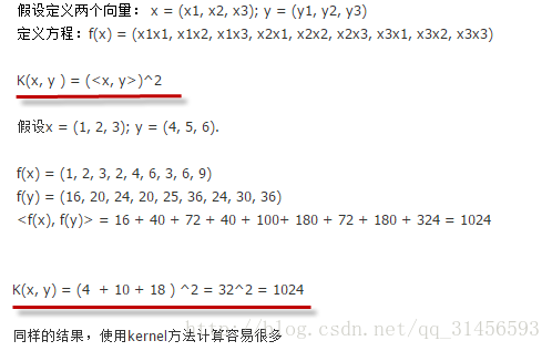
核函式舉例
程式碼
# -*- coding: utf-8 -*-
from sklearn import svm
# 資料
x = [[2, 0], [1, 1], [2, 3]]
# 標籤
y = [0, 0, 1]
# 線性可分的svm分類器,用線性的核函式
clf = svm.SVC(kernel='linear' # -*- coding: utf-8 -*-
import numpy as np
import pylab as pl
from sklearn import svm
np.random.seed(0) # 值固定,每次隨機結果不變
# 2組20 # -*- coding: utf-8 -*-
from __future__ import print_function
from time import time
import logging # 列印程式進展的資訊
import matplotlib.pyplot as plt
from sklearn.cross_validation import train_test_split
from sklearn.datasets import fetch_lfw_people
from sklearn.grid_search import GridSearchCV
from sklearn.metrics import classification_report
from sklearn.metrics import confusion_matrix
from sklearn.decomposition import RandomizedPCA
from sklearn.svm import SVC
print(__doc__)
# 列印程式進展的資訊
logging.basicConfig(level=logging.INFO, format='%(asctime)s %(message)s')
###############################################################################
# 下載人臉資料集,並匯入
lfw_people = fetch_lfw_people(min_faces_per_person=70, resize=0.4)
# 資料集多少,長寬多少
n_samples, h, w = lfw_people.images.shape
# x是特徵向量的矩陣,獲取矩陣列數,即緯度
X = lfw_people.data
n_features = X.shape[1]
# y是分類標籤向量
y = lfw_people.target
# 類別裡面有誰的名字
target_names = lfw_people.target_names
# 名字有多少行,即有多少人要區分
n_classes = target_names.shape[0]
# 列印
print("Total dataset size:")
print("n_samples: %d" % n_samples)
print("n_features: %d" % n_features)
print("n_classes: %d" % n_classes)
###############################################################################
# 將資料集劃分為訓練集和測試集,測試集佔0.25
X_train, X_test, y_train, y_test = train_test_split(
X, y, test_size=0.25)
###############################################################################
# PCA降維
n_components = 150 # 組成元素數量
print("Extracting the top %d eigenfaces from %d faces"
% (n_components, X_train.shape[0]))
t0 = time()
# 建立PCA模型
pca = RandomizedPCA(n_components=n_components, whiten=True).fit(X_train)
print("done in %0.3fs" % (time() - t0))
# 提取特徵臉
eigenfaces = pca.components_.reshape((n_components, h, w))
print("Projecting the input data on the eigenfaces orthonormal basis")
t0 = time()
# 將特徵向量轉化為低維矩陣
X_train_pca = pca.transform(X_train)
X_test_pca = pca.transform(X_test)
print("done in %0.3fs" % (time() - t0))
###############################################################################
# Train a SVM classification model
print("Fitting the classifier to the training set")
t0 = time()
# C錯誤懲罰權重 gamma 建立核函式的不同比例
param_grid = {'C': [1e3, 5e3, 1e4, 5e4, 1e5],
'gamma': [0.0001, 0.0005, 0.001, 0.005, 0.01, 0.1], }
# 選擇核函式,建SVC,嘗試執行,獲得最好引數
clf = GridSearchCV(SVC(kernel='rbf', class_weight='auto'), param_grid)
# 訓練
clf = clf.fit(X_train_pca, y_train)
print("done in %0.3fs" % (time() - t0))
print("Best estimator found by grid search:")
print(clf.best_estimator_) # 輸出最佳引數
###############################################################################
# Quantitative evaluation of the model quality on the test set
print("Predicting people's names on the test set")
t0 = time()
# 預測
y_pred = clf.predict(X_test_pca)
print("done in %0.3fs" % (time() - t0))
print(classification_report(y_test, y_pred, target_names=target_names)) # 與真實情況作對比求置信度
print(confusion_matrix(y_test, y_pred, labels=range(n_classes))) # 對角線的為預測正確的,a預測為a
###############################################################################
# Qualitative evaluation of the predictions using matplotlib
def plot_gallery(images, titles, h, w, n_row=3, n_col=4):
"""Helper function to plot a gallery of portraits"""
plt.figure(figsize=(1.8 * n_col, 2.4 * n_row))
plt.subplots_adjust(bottom=0, left=.01, right=.99, top=.90, hspace=.35)
for i in range(n_row * n_col):
plt.subplot(n_row, n_col, i + 1)
plt.imshow(images[i].reshape((h, w)), cmap=plt.cm.gray)
plt.title(titles[i], size=12)
plt.xticks(())
plt.yticks(())
# plot the result of the prediction on a portion of the test set
def title(y_pred, y_test, target_names, i):
pred_name = target_names[y_pred[i]].rsplit(' ', 1)[-1]
true_name = target_names[y_test[i]].rsplit(' ', 1)[-1]
return 'predicted: %s\ntrue: %s' % (pred_name, true_name)
prediction_titles = [title(y_pred, y_test, target_names, i)
for i in range(y_pred.shape[0])]
plot_gallery(X_test, prediction_titles, h, w) # 畫出測試集和它的title
# plot the gallery of the most significative eigenfaces
eigenface_titles = ["eigenface %d" % i for i in range(eigenfaces.shape[0])]
plot_gallery(eigenfaces, eigenface_titles, h, w) # 列印特徵臉
plt.show() # 顯示