Overview

The Geometry of Linear Equations

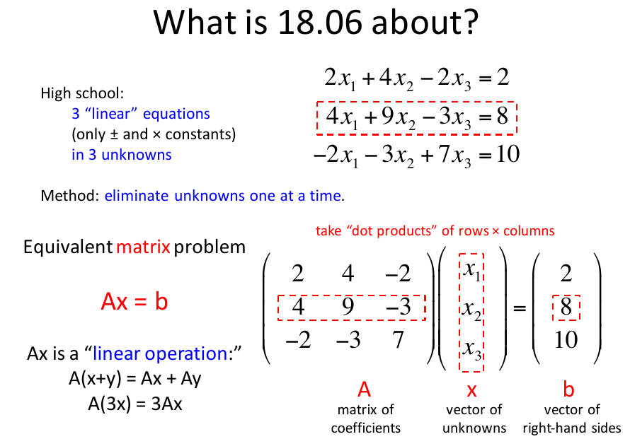
教授在這個 lecture 中介紹了3個概念：Row Picture，Column Picture, and Matrix Picture，其中理解 Column Picture 是最重要的。

我們可以把線性方程組寫成矩陣的形式，Row Picture 描述的是從矩陣的 row 看起，對於每一個 row 來說，在 2D 中可以決定一條直線，在 3D 中決定一個平面; 而對於 Column Picture 來說，從 column 看起，形成了列向量的 linear combination

，因此在 2D 和 3D 中都是向量，只不過2者之間相差一個維度而已; Matrix Picture 沒什麼好說的。詳情可以看 The Geometry of Linear Equations.

Given a matrix A, can we solve: Ax=b for every possible vector b? In other words, do the linear combinations of the column vectors fill the xy-plane (or space, in the three dimensional case)?

If the answer is “no”, we say that A

is a singular matrix. In this singular case its column vectors are linearly dependent; all linear combinations of those vectors lie on a point or line in two dimensions(plane in three dimensions). The combinations don’t fill the whole space.

從幾何上理解會更直觀一些。比如在空間中有3個向量（A，B，C），如果 A 和 B 通過 linear combination 會得到 C，因此 C 在向量 A 與 B 組成的平面上，因此這3個向量的 linear combinations 不能 fill 整個3維空間。在進一步，如果這3個向量共線，那麼它們就只能 fill 一條直線。

Elimination with Matrices

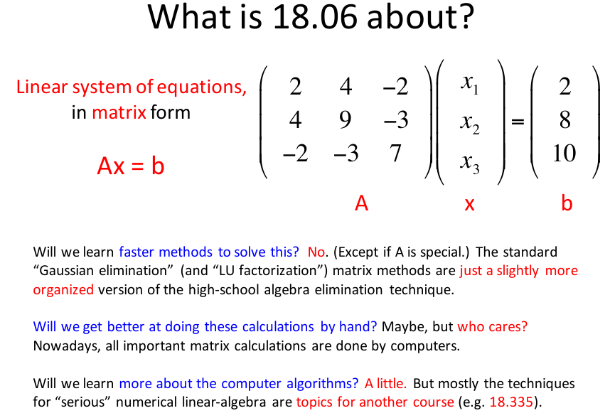
在文章開頭，已經看到了線性方程組可以寫成矩陣的形式。下圖中就是把一個3元方程組寫成矩陣的形式（Ax=b）：

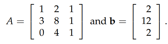
在高中的時候，如果想要求解出這樣的方程組，需要不斷地化簡消元，只不過我們現在用更加系統的方法去做這件事情，道理本身是一樣的。這裡直接操縱矩陣，從而達到消元的目的。過程如下圖所示：

由於對方程的左邊（即矩陣 A）進行了上述步驟的簡化，同樣的步驟也需要應用到向量 b 上。應用到 b 以後，我們得到了一個新的向量 c=⎡⎣⎢26−10⎤⎦⎥，因此整個消元方法轉換 Ax=b 到 Ux=c，通過 back substitution 就可以得到這個3元方程組的解了。

在上面的消元過程中，pivots may not be 0. If there is a zero in the pivot position, we must exchange that row with one below to get a non-zero value in the pivot position. If there is a zero in the pivot position and no non-zero value below it, then the matrix A is not invertible.

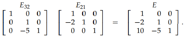
熟悉了上面的消元過程，現在讓我們瞭解一下 Elimination Matrices 的概念。在上面消元的第一步中，我們是把矩陣 A 的 row 2 - 3×row 1，通過下圖中的方式也可以達到同樣的效果：

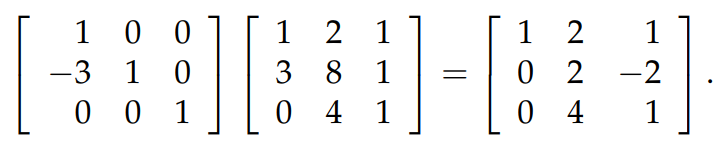
上圖中最左面的矩陣就是消元矩陣。The elimination matrix used to eliminate the entry in row m column n is denoted Emn. The calculation above took us from A to E21A. The three elimination steps leading to U were: E32(E31(E21A))=U. 這裡你會發現一個關於 elimination matrix 的規律，構成一個 elimination matrix，首先寫一個單位矩陣，然後如果你想消哪個位置的元素，然後改變這個單位矩陣相對應的位置的值，使其達到消元的目的。你可以動手試一試。

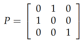
A permutation matrix exchanges two rows of a matrix. 對於一個 n×n 的矩陣來說，可以有 n! 種方式交換行，因此就有 n! 個permutation matrix，這些矩陣形成了一個組. 單位矩陣就是一個 permutation matrix 的例子，只不過它不交換任何行而已。關於 permutation matrix 的規律，就是你怎樣交換單位矩陣的行，你就如何交換另一個應用到它的矩陣的行。比如對於下圖中的 permutation matrix 來說，它交換了單位矩陣的行1和行2，如果你把這個 permutation matrix 應用到另一個矩陣上，那麼它就會交換那個矩陣的第1行和第2行。

既然我們有 n! 種方式交換行，無論你怎麼交換都逃不出這些可能。因此，無論你對同一個矩陣應用多少個 permutation matrix，交換之後的結果一定在 n! 種情況內。因此可以得出，當你從一組 permutation matrix 中拿出任意多個矩陣時，它們的乘積也一定在組裡。

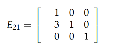
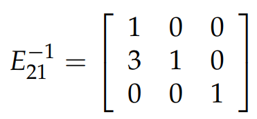
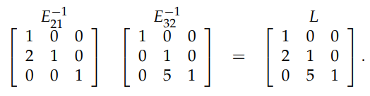
接下來我再談一下關於 elimination matrix 的逆矩陣。比如下圖中的 elimination matrix，它的目的是進行操作： row 2 - 3×row 1，為了 “undo” 這個操作，我們必須進行操作： row 2 -+3×row 1，即用 E21 的逆矩陣：

Multiplication and Inverse Matrices

有5種 perspective 來看矩陣的乘法：它們分別是：row times column，columns，rows，column times row，blocks. 關於它們的詳情參考 矩陣乘法。

接下來談一談如何判斷 square matrix A 是否可逆。設矩陣 Ax=0，如果你可以找到一個非0的 x 使其成立，則 A 不可逆。這是為什麼呢？假設 A−1 存在，且有一個非0解 x. 由於 A−1(Ax)=A−10=0≠x=Ix=(A−1A)x，違背了假設，所以矩陣 A 不可逆。

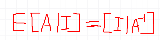
接下來談一談當一個矩陣可逆的時候，如何用 Gauss-Jordan Elimination 來求出它的逆矩陣。下圖中就是整個過程（Once we have used Gauss’ elimination method to convert the original matrix to upper triangular form, we go on to use Jordan’s idea of eliminating entries in the upper right portion of the matrix）。

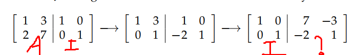
上面的消元過程很好理解，但是為什麼上圖中“問號”上面的矩陣就是 A−1 呢？在下圖中通過把一個 elimination matrix E 應用到矩陣 A 上得到了單位矩陣 I，即 EA=I，所以 E=A−1，所以 EI=A−1I=A−1

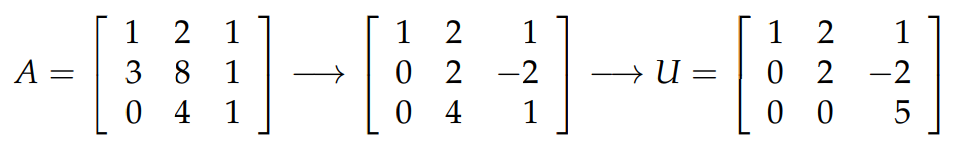
Factorization into A = LU

正如本節標題所示，我們需要把矩陣 A 分解成2個矩陣（L 和 U）的乘積，where ‘LU’ stands for ‘lower upper’, and also called LU factorization. 在上面的小節中已經看到，通過對矩陣 A 的消元過程，最終可以得到一個 upper triangular 的矩陣 U，因此是 EA=U. 有了過程，我們就可以很容易把 A 分解成 LU 了。E−1EA=E−1U，因此你會發現 L 實際上就是 E−1.

矩陣 L 是 lower triangular 的，而且對角線上全是1. 你可以看每一步的消元矩陣，它都是對角線上是1，然後改變某個位置上的乘子。你可能會想，A=LU 和 EA=U，並沒有什麼太大區別嗎！我們為什麼更傾向於前者呢？舉個例子一下就明白了。比如某個矩陣 A 的 A21 和 A32 兩個元素需要消元，因此有下圖中的2個消元矩陣。你會發現最終得到的 E 不僅在其需要消元的2個元素上有乘子，而且在左下角不還有個10出現，這就是副作用。

而對於通過求消元矩陣的逆，從而得到的 L 來說，如下圖所示，它並沒有這樣的副作用。因此在沒有行交換的情況下，消元矩陣中的乘子可以直接複製到 L 中。

當需要交換行時，我們可以寫成：PA=LU，其中的 P 是 permutation matrix. 這種型別的矩陣有很好的性質：P−1=PT

A matrix A is symmetric if AT=A. Given any matrix R (not necessarily square) the product RTR is always symmetric, because (RTR)T=RT(RT)T=RTR

Vector Spaces

來自維基百科的定義：

A vector space (also called a linear space) is a collection of objects called vectors, which may be added together and multiplied (“scaled”) by numbers, called scalars.

通過上面的定義，我們可以判斷一個給定的向量集合是否為 vector space. 比如，在 x-y 平面上第1象限的向量集合，它就不是 vector space. 集合中的任意2個向量相加依然在集合中，但是如果你乘上一個負數，得到的向量就不在集合中了。我們說這種型別的向量集合是 closed under addition but not under multiplication.

關於 subspace 的定義：

A vector space that is contained inside of another vector space is called a subspace of that space. Every subspace must contain the zero vector because vector spaces are closed under multiplication.

下面舉2個例子：

1. The subspaces of R2

   • all of R2
   • any line through the origin
   • the zero vector alone

2. The subspaces of R3

   • all of R3
   • any plane through the origin
   • any line through the origin
   • the zero vector alone

Column Space and Nullspace

對於一個 m×n 的矩陣 A 來說，column space 和 nullspace 是2個非常重要的 subspace，because they tell us a lot about the matrix A and solutions to Ax=b.

column space 的定義：

The column space of a matrix A is the vector space made up of all linear combinations of the columns of A.

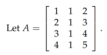
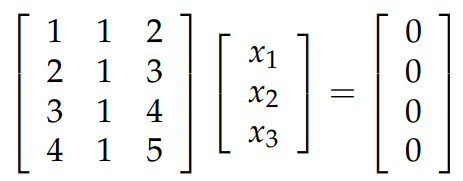
從上面的定義可以知道，如果線性方程組 Ax=b 有解，那麼向量 b 必須要在矩陣 A 的 column space 上。比如對於下圖中的矩陣 A 來說，什麼樣的向量 b 可以使得 Ax=b 有解？不難發現，A 的第3列不是 independent 的，它是前2列的和，因此矩陣 A 的 column space 是4維枯空間中的 2D 的子空間，即一個過原點的平面。因此，只有在這個平面上的向量 b，我們才可以得到解。

nullspace 的定義：

The nullspace of a matrix A is the collection of all solutions x to the equation Ax = 0

你可能會想，nullspace 為什麼會是 vector space 呢？我們假設 Ax=0 的解為向量 x; 這會導致 cx 也是解，因為 A(cx)=cAx=0; 同樣道理 x1+x2 也會是解，因為 A(x1+x2)=Ax1+Ax2=0。比如下圖中的例子，我們一下就可以看出 x=⎡⎣⎢11−1⎤⎦⎥ 是其中的一個解，因此 cx 也會是解，所有的這些解構成了 nullspace，對於這個題目來說，nullspace 是三維空間中的一條過原點的直線。

Solving Ax = 0

上面我們已經介紹了一個矩陣的 nullspace 是什麼，那麼如何來計算出它呢？Khan 學院中的 Calculating the null space of a matrix 拿一個具體的例子來講解找 null space 的過程。下面我來總結一下 MIT 課上介紹的方法，其實它們本質都是一樣的。

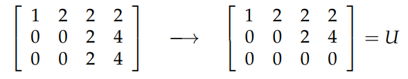
那麼如何求下圖矩陣 A 的 null space 呢？首先，需要通過消元把矩陣 A 化簡成 reduced row echelon form（它的 pivots 等於1，pivots 的上下全是0），在消元的過程中，它並不會改變 Ax=b 的解，因此就不會改變 null space.

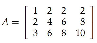
下圖中的消元過程使得矩陣 A 轉化成了 U. 矩陣的 rank 等於它所擁有的 pivots 的數量，在這個例子中，rank=2. 我們把包含 pivot 的列叫做 pivot columns，剩下的列叫做 free columns，在我們這個例子中，第1和第3列為 pivot columns，第2和第4列為 free columns. 至此，我們已經把 Ax=0 的問題轉換成了 Ux=0 的問題。

接下來，我們繼續消元，把 U 化簡成 reduced row echelon form，如下圖所示。得到了 R 以後，我們就可以很容易地求出 null space 了。

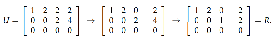
通過交換 R 中的一些列，我們可以把上面的 R 改寫成下圖所示的 block matrix. 上面已經說過了，這個矩陣的 rank 為2，而下圖中的 I 是包含 pivot 的列，因此 I 是一個 2×2 的方陣; 由於總共的列數為4，free columns 為4-2=2，因此 F