
CS229 6.3 Neurons Networks Gradient Checking
BP演算法很難除錯,一般情況下會隱隱存在一些小問題,比如(off-by-one error),即只有部分層的權重得到訓練,或者忘記計算bais unit,這雖然會得到一個正確的結果,但效果差於準確BP得到的結果。
有了cost function,目標是求出一組引數W,b,這裡以 表示,cost function 暫且記做
 。假設
。假設  ,則
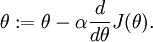
,則  ,即一維情況下的Gradient Descent:
根據6.2中對單個引數單個樣本的求導公式:
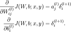
可以得到每個引數的偏導數,對所有樣本累計求和,可以得到所有訓練資料對引數 的偏導數記做  , 是靠BP演算法求得的,為了驗證其正確性,看下圖回憶導數公式:
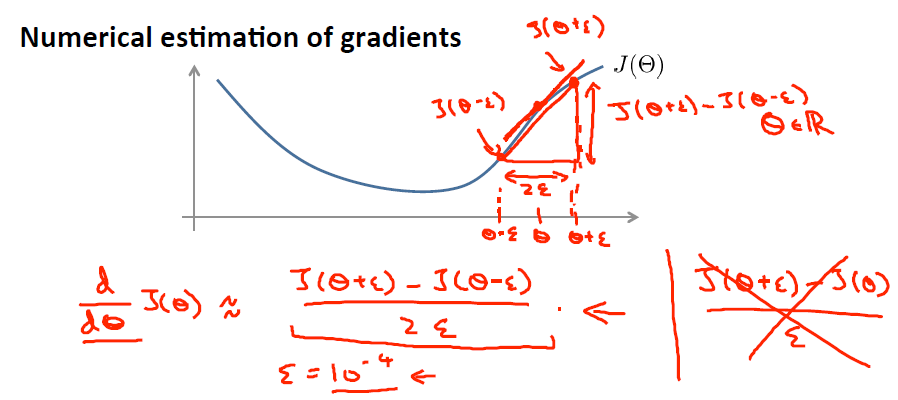
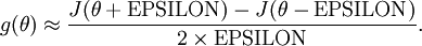
可見有: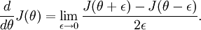 那麼對於任意 值,我們都可以對等式左邊的導數用:
 來近似。
來近似。
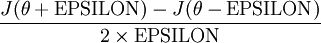
給定一個被認為能計算  的函式,可以用下面的數值檢驗公式
應用時,通常把 設定為一個很小的常量,比如在
 數量級,最好不要太小了,會造成數值的舍入誤差。上式兩端值的接近程度取決於
  的具體形式。假定
 的情況下,上式左右兩端至少有4位有效數字是一樣的(通常會更多)。
當 是一個n維向量而不是實數時,且
  ,在 Neorons Network 中,J(W,b)可以想象為 W,b 組合擴充套件而成的一個長向量
 的函式
的函式  ,如何檢驗能否輸出到正確結果呢,用的取值來檢驗,對於向量的偏導數:
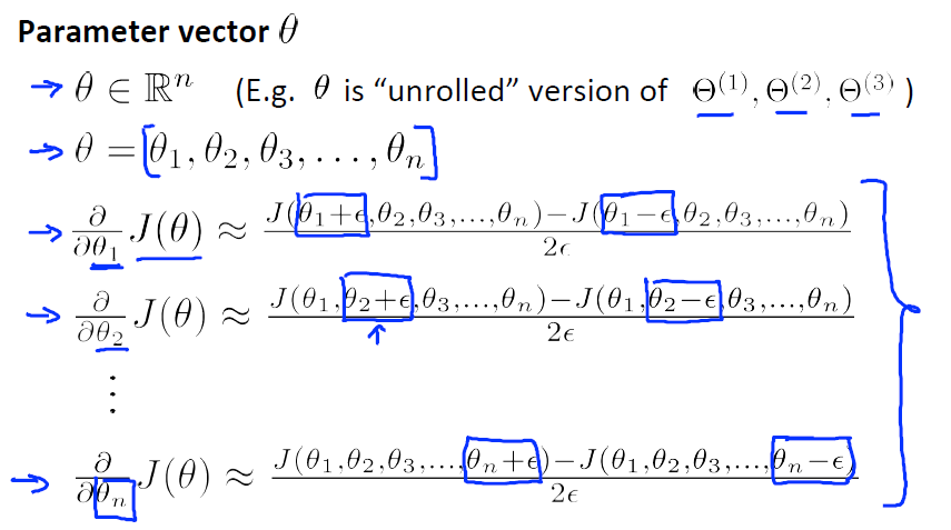
根據上圖,對 i 求導時,只需要在向量的第i維上進行加減操作,然後求值即可,定義  ,其中
,其中
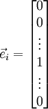
 和 幾乎相同,除了第
  行元素增加了 ,類似地,
 得到的第 行減小了 ,然後求導並與比較:
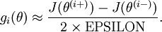
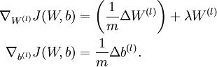
 中的引數對應的是引數向量中一個分量的細微變化,損失函式J 在不同情況下會有不同的值(比如三層NN 或者 三層autoencoder(需加上稀疏項)),上式中左邊為BP演算法的結果,右邊為真正的梯度,只要兩者很接近,說明BP演算法是在正確工作,對於梯度下降中的引數是按照如下方式進行更新的:
![\begin{align}
W^{(l)} &= W^{(l)} - \alpha \left[ \left(\frac{1}{m} \Delta W^{(l)} \right) + \lambda W^{(l)}\right] \\
b^{(l)} &= b^{(l)} - \alpha \left[\frac{1}{m} \Delta b^{(l)}\right]
\end{align}](http://ufldl.stanford.edu/wiki/images/math/0/f/7/0f7430e97ec4df1bfc56357d1485405f.png)
即有 分別為:
最後只需總體損失函式J(W,b)的偏導數與上述 的值比較即可。
除了梯度下降外,其他的常見的優化演算法:1) 自適應 的步長,2) BFGS L-BFGS,3) SGD,4) 共軛梯度演算法,以後涉及到再看。