
CS229 6.10 Neurons Networks implements of softmax regression
阿新 • • 發佈:2018-11-27
softmax可以看做只有輸入和輸出的Neurons Networks,如下圖:

其引數數量為k*(n+1) ,但在本實現中沒有加入截距項,所以引數為k*n的矩陣。
對損失函式J(θ)的形式有:
![\begin{align}
J(\theta) = - \frac{1}{m} \left[ \sum_{i=1}^{m} \sum_{j=1}^{k} 1\left\{y^{(i)} = j\right\} \log \frac{e^{\theta_j^T x^{(i)}}}{\sum_{l=1}^k e^{ \theta_l^T x^{(i)} }} \right]
+ \frac{\lambda}{2} \sum_{i=1}^k \sum_{j=0}^n \theta_{ij}^2
\end{align}](http://ufldl.stanford.edu/wiki/images/math/4/7/1/471592d82c7f51526bb3876c6b0f868d.png)
演算法步驟:
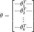
首先,載入資料集{x(1),x(2),x(3)...x(m)}該資料集為一個n*m的矩陣,然後初始化引數 θ ,為一個k*n的矩陣(不考慮截距項):

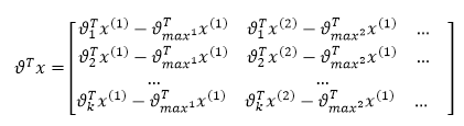
首先計算 ,該矩陣為k*m的:

然後計算 :
:
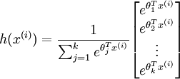
該函式引數可以隨意+-任意引數而保持值不變,所以為了防止 引數 過大,先減去一個常量,防止資料運算時產生溢位.
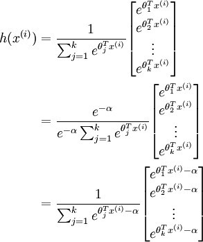
這裡減去每一類的最大值, 代表第i列最大值。
對於上述矩陣,每列除以該列的總和,並且取log即可求得其歸一化後的概率,用P來表示,上述矩陣的每一列表示訓練資料 分別屬於類別k的概率,每一列的和為1.
下面計算Ground Truth 矩陣,該矩陣即代表了損失函式中的: ,Ground Truth 矩陣為k*m的矩陣,每一列代表一個標籤,該列中除第k行為1外,其他的元素均為0,k即為該列標籤對應的值,比如對於K=4時,的四個樣本:

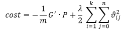
上圖代表了 ,把上述矩陣擴充套件為k*m即可。用符號G來表示該矩陣,即可得到下面的cost function:
下面需要對損失函式求導,來得到:
![\begin{align}
\nabla_{\theta_j} J(\theta) = - \frac{1}{m} \sum_{i=1}^{m}{ \left[ x^{(i)} ( 1\{ y^{(i)} = j\} - p(y^{(i)} = j | x^{(i)}; \theta) ) \right] } + \lambda \theta_j
\end{align}](http://ufldl.stanford.edu/wiki/images/math/3/a/f/3afb4b9181a3063ddc639099bc919197.png)
以上公式得到一個k*n的矩陣,每一列即為對引數 的導數。
的導數。

接下來梯度檢驗,驗證上一句的正確性,若正確,則用L-BFGS求解最優解,直接用最優解來進行預測即可。下面是matlab程式碼:


%% STEP 0: 初始化引數與常量 % % Here we define and initialise some constants which allow your code % to be used more generally on any arbitrary input. % We also initialise some parameters used for tuning the model. inputSize =View Code28 * 28; % Size of input vector (MNIST images are 28x28) numClasses = 10; % Number of classes (MNIST images fall into 10 classes) lambda = 1e-4; % Weight decay parameter %%====================================================================== %% STEP 1: Load data % % In this section, we load the input and output data. % For softmax regression on MNIST pixels, % the input data is the images, and % the output data is the labels. % % Change the filenames if you've saved the files under different names % On some platforms, the files might be saved as % train-images.idx3-ubyte / train-labels.idx1-ubyte images = loadMNISTImages('mnist/train-images-idx3-ubyte'); labels = loadMNISTLabels('mnist/train-labels-idx1-ubyte'); labels(labels==0) = 10; % 注意下標是1-10,所以需要 把0對映到10 inputData = images; % For debugging purposes, you may wish to reduce the size of the input data % in order to speed up gradient checking. % Here, we create synthetic dataset using random data for testing DEBUG = true; % Set DEBUG to true when debugging. if DEBUG inputSize = 8; inputData = randn(8, 100);%randn產生每個元素均為標準正態分佈的8*100的矩陣 labels = randi(10, 100, 1);%產生1-10的隨機數,產生100行,即100個標籤 end % Randomly initialise theta theta = 0.005 * randn(numClasses * inputSize, 1); %%====================================================================== %% STEP 2: Implement softmaxCost % % Implement softmaxCost in softmaxCost.m. [cost, grad] = softmaxCost(theta, numClasses, inputSize, lambda, inputData, labels); %%====================================================================== %% STEP 3: Gradient checking % % As with any learning algorithm, you should always check that your % gradients are correct before learning the parameters. % % h = @(x) scale * kernel(scale * x); % 構建一個自變數為x,因變數為h,表示式為scale * kernel(scale * x)的函式。即 % h=scale* kernel(scale * x),自變數為x if DEBUG numGrad = computeNumericalGradient( @(x) softmaxCost(x, numClasses, ... inputSize, lambda, inputData, labels), theta); % Use this to visually compare the gradients side by side disp([numGrad grad]); % Compare numerically computed gradients with those computed analytically diff = norm(numGrad-grad)/norm(numGrad+grad); disp(diff); % The difference should be small. % In our implementation, these values are usually less than 1e-7. % When your gradients are correct, congratulations! end %%====================================================================== %% STEP 4: Learning parameters % % Once you have verified that your gradients are correct, % you can start training your softmax regression code using softmaxTrain % (which uses minFunc). options.maxIter = 100; softmaxModel = softmaxTrain(inputSize, numClasses, lambda, ... inputData, labels, options); % Although we only use 100 iterations here to train a classifier for the % MNIST data set, in practice, training for more iterations is usually % beneficial. %%====================================================================== %% STEP 5: Testing % % You should now test your model against the test images. % To do this, you will first need to write softmaxPredict % (in softmaxPredict.m), which should return predictions % given a softmax model and the input data. images = loadMNISTImages('mnist/t10k-images-idx3-ubyte'); labels = loadMNISTLabels('mnist/t10k-labels-idx1-ubyte'); labels(labels==0) = 10; % Remap 0 to 10 inputData = images; % You will have to implement softmaxPredict in softmaxPredict.m [pred] = softmaxPredict(softmaxModel, inputData); acc = mean(labels(:) == pred(:)); fprintf('Accuracy: %0.3f%%\n', acc * 100); % Accuracy is the proportion of correctly classified images % After 100 iterations, the results for our implementation were: % % Accuracy: 92.200% % % If your values are too low (accuracy less than 0.91), you should check % your code for errors, and make sure you are training on the % entire data set of 60000 28x28 training images % (unless you modified the loading code, this should be the case) end %%%%對應STEP 2: Implement softmaxCost function [cost, grad] = softmaxCost(theta, numClasses, inputSize, lambda, data, labels) % numClasses - the number of classes % inputSize - the size N of the input vector % lambda - weight decay parameter % data - the N x M input matrix, where each column data(:, i) corresponds to % a single test set % labels - an M x 1 matrix containing the labels corresponding for the input data theta = reshape(theta, numClasses, inputSize);% 轉化為k*n的引數矩陣 numCases = size(data, 2);%或者data矩陣的列數,即樣本數 % M = sparse(r, c, v) creates a sparse matrix such that M(r(i), c(i)) = v(i) for all i. % That is, the vectors r and c give the position of the elements whose values we wish % to set, and v the corresponding values of the elements % labels = (1,3,4,10 ...)^T % 1:numCases=(1,2,3,4...M)^T % sparse(labels, 1:numCases, 1) 會產生 % 一個行列為下標的稀疏矩陣 % (1,1) 1 % (3,2) 1 % (4,3) 1 % (10,4) 1 %這樣改矩陣填滿後會變成每一列只有一個元素為1,該元素的行即為其lable k %1 0 0 ... %0 0 0 ... %0 1 0 ... %0 0 1 ... %0 0 0 ... %. . . %上矩陣為10*M的 ,即 groundTruth 矩陣 groundTruth = full(sparse(labels, 1:numCases, 1)); cost = 0; % 每個引數的偏導數矩陣 thetagrad = zeros(numClasses, inputSize); % theta(k*n) data(n*m) %theta * data = k*m , 第j行第i列為theta_j^T * x^(i) %max(M)產生一個行向量,每個元素為該列中的最大值,即對上述k*m的矩陣找出m列中每列的最大值 M = bsxfun(@minus,theta*data,max(theta*data, [], 1)); % 每列元素均減去該列的最大值,見圖- M = exp(M); %求指數 p = bsxfun(@rdivide, M, sum(M)); %sum(M),對M中的元素按列求和 cost = -1/numCases * groundTruth(:)' * log(p(:)) + lambda/2 * sum(theta(:) .^ 2);%損失函式值 %groundTruth 為k*m ,data'為m*n,即theta為k*n的矩陣,n代表輸入的維度,k代表類別,即沒有隱層的 %輸入為n,輸出為k的神經網路 thetagrad = -1/numCases * (groundTruth - p) * data' + lambda * theta; %梯度,為 k * % ------------------------------------------------------------------ % Unroll the gradient matrices into a vector for minFunc grad = [thetagrad(:)]; end %%%%對應STEP 3: Implement softmaxCost % 函式的實際引數是這樣的J = @(x) softmaxCost(x, numClasses, inputSize, lambda, inputData, labels) % 即函式的形式引數J以x為自變數,別的都是以預設的值為相應的變數 function numgrad = computeNumericalGradient(J, theta) % theta: 引數,向量或者實數均可 % J: 輸出值為實數的函式. 呼叫y = J(theta)將會返回函式在theta處的值 % numgrad初始化為0,與theta維度相同 numgrad = zeros(size(theta)); EPSILON = 1e-4; % theta是一個行向量,size(theta,1)是求行數 n = size(theta,1); %產生一個維度為n的單位矩陣 E = eye(n); for i = 1:n % (n,:)代表第n行,所有的列 % (:,n)代表所有行,第n列 % 由於E是單位矩陣,所以只有第i行第i列的元素變為EPSILON delta = E(:,i)*EPSILON; %向量第i維度的值 numgrad(i) = (J(theta+delta)-J(theta-delta))/(EPSILON*2.0); end %%%%對應STEP 4: Implement softmaxCost function [softmaxModel] = softmaxTrain(inputSize, numClasses, lambda, inputData, labels, options) %softmaxTrain Train a softmax model with the given parameters on the given % data. Returns softmaxOptTheta, a vector containing the trained parameters % for the model. % % inputSize: the size of an input vector x^(i) % numClasses: the number of classes % lambda: weight decay parameter % inputData: an N by M matrix containing the input data, such that % inputData(:, i) is the ith input % labels: M by 1 matrix containing the class labels for the % corresponding inputs. labels(c) is the class label for % the cth input % options (optional): options % options.maxIter: number of iterations to train for if ~exist('options', 'var') options = struct; end if ~isfield(options, 'maxIter') options.maxIter = 400; end % initialize parameters,randn(M,1)產生均值為0,方差為1長度為M的陣列 theta = 0.005 * randn(numClasses * inputSize, 1); % Use minFunc to minimize the function addpath minFunc/ options.Method = 'lbfgs'; % Here, we use L-BFGS to optimize our cost % function. Generally, for minFunc to work, you % need a function pointer with two outputs: the % function value and the gradient. In our problem, % softmaxCost.m satisfies this. minFuncOptions.display = 'on'; [softmaxOptTheta, cost] = minFunc( @(p) softmaxCost(p, ... numClasses, inputSize, lambda, ... inputData, labels), ... theta, options); % Fold softmaxOptTheta into a nicer format softmaxModel.optTheta = reshape(softmaxOptTheta, numClasses, inputSize); softmaxModel.inputSize = inputSize; softmaxModel.numClasses = numClasses; end %%%%對應 STEP 5: Implement predict function [pred] = softmaxPredict(softmaxModel, data) % softmaxModel - model trained using softmaxTrain % data - the N x M input matrix, where each column data(:, i) corresponds to % a single test set % % Your code should produce the prediction matrix % pred, where pred(i) is argmax_c P(y(c) | x(i)). % Unroll the parameters from theta theta = softmaxModel.optTheta; % this provides a numClasses x inputSize matrix pred = zeros(1, size(data, 2)); %C = max(A) %返回一個數組各不同維中的最大元素。 %如果A是一個向量,max(A)返回A中的最大元素。 %如果A是一個矩陣,max(A)將A的每一列作為一個向量,返回一行向量包含了每一列的最大元素。 %根據預測函式找出每列的最大值即可。 [nop, pred] = max(theta * data); end