
CS229 6.9 Neurons Networks softmax regression
SoftMax迴歸模型,是logistic迴歸在多分類問題的推廣,即現在logistic迴歸資料中的標籤y不止有0-1兩個值,而是可以取k個值,softmax迴歸對諸如MNIST手寫識別庫等分類很有用,該問題有0-9 這10個數字,softmax是一種supervised learning方法。
在logistic中,訓練集由  個已標記的樣本構成:
 ,其中輸入特徵
 (特徵向量
(特徵向量  的維度為
的維度為  ,其中
,其中  對應截距項 ), logistic 迴歸是針對二分類問題的,因此類標記
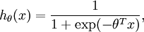
  。假設函式(hypothesis function) 如下:
損失函式為負log損失函式:
![\begin{align}
J(\theta) = -\frac{1}{m} \left[ \sum_{i=1}^m y^{(i)} \log h_\theta(x^{(i)}) + (1-y^{(i)}) \log (1-h_\theta(x^{(i)})) \right]
\end{align}](http://ufldl.stanford.edu/wiki/images/math/f/a/6/fa6565f1e7b91831e306ec404ccc1156.png)
找到使得損失函式最小時的模型引數  ,帶入假設函式即可求解模型。
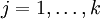
在softmax迴歸中,對於訓練集 中的類標  可以取
可以取  個不同的值(而不是 2 個),即有
 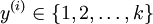 (注意不是由0開始), 在MNIST中有K=10個類別。
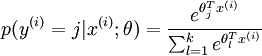
在softmax迴歸中,對於輸入x,要計算x分別屬於每個類別j的概率 ,即求得x分別屬於每一類的概率,因此假設函式要設定為輸出一個k維向量,每個維度代表x被分為每個類別的概率,假設函式
  形式如下:
形式如下:
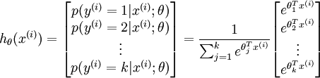
請注意  這一項對概率分佈進行歸一化,使得所有概率之和為 1 。當類別數
時,softmax 迴歸的假設函式為: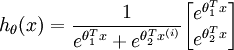 ,對該式進行化簡得到:
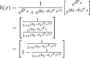
另  來表示
來表示 ,我們就會發現 softmax 迴歸器預測其中一個類別的概率為
  ,另一個類別概率的為
 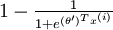 ,這與 logistic迴歸是一致的。
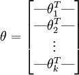
其中  是模型的引數。把引數 表示為矩陣形式有, 是一個
  的矩陣,該矩陣是將
  按行羅列起來得到的:
有個假設函式(Hypothesis Function),下面來看代價函式,根據代價函式求解出最優引數值帶入假設函式即可求得最終的模型,先引入函式 ,對於該函式有:
 值為真的表示式
  值為假的表示式
  。
。
舉例來說,表示式  的值為1 ,
 的值為 0 。
則softmax的損失函式為:
![\begin{align}
J(\theta) = - \frac{1}{m} \left[ \sum_{i=1}^{m} \sum_{j=1}^{k} 1\left\{y^{(i)} = j\right\} \log \frac{e^{\theta_j^T x^{(i)}}}{\sum_{l=1}^k e^{ \theta_l^T x^{(i)} }}\right]
\end{align}](http://ufldl.stanford.edu/wiki/images/math/7/6/3/7634eb3b08dc003aa4591a95824d4fbd.png)
當k=2時,即有logistic的形式,下邊是推倒:
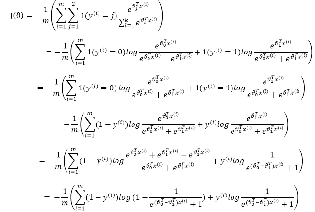
另上式中的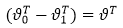 便得到了logistic迴歸的損失函式。
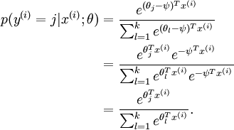
可以看到,softmax與logistic的損失函式只是k的取值不同而已,且在softmax中將類別x歸為類別j的概率為:
 .
.
需要注意的一個問題是softmax迴歸中的模型引數化問題,即softmax的引數集是“冗餘的”。
假設從引數向量  中減去了向量
  ,這時,每一個 都變成了
  (
( )。此時假設函式變成了以下的式子:
也就是說,從 中減去 完全不影響假設函式的預測結果,這就說明 Softmax 模型被過度引數化了。對於任意一個用於擬合數據的假設函式,可以求出多組引數值,這些引數得到的是完全相同的假設函式  ,也就是說如果引數集合
  是代價函式
是代價函式  的極小值點,那麼
 同樣也是它的極小值點,其中 可以是任意向量,到底是什麼造成的呢?從巨集觀上可以這麼理解,因為此時的損失函式不是嚴格非凸的,也就是說在區域性最小值點附近是一個”平坦”的,所以在這個引數附近的值都是一樣的了。平坦假設函式空間的Hessian 矩陣是奇異的/不可逆的,這會直接導致採用牛頓法優化就遇到數值計算的問題。因此使 最小化的解不是唯一的。但此時 仍然是一個凸函式,因此梯度下降時不會遇到區域性最優解的問題。
還有一個值得注意的地方是:當  時,我們總是可以將
  替換為
替換為 (即替換為全零向量),並且這種變換不會影響假設函式。因此我們可以去掉引數向量 (或者其他 中的任意一個)而不影響假設函式的表達能力。實際上,與其優化全部的 個引數 (其中
  ),我們可以令
  ,只優化剩餘的
  個引數,這樣演算法依然能夠正常工作。比如logistic就是這樣的。
在實際應用中,為了使演算法看起來更直觀更清楚,往往保留所有引數  ,而不任意地將某一引數設定為 0。但此時需要對代價函式做一個改動:加入權重衰減。權重衰減可以解決 softmax 迴歸的引數冗餘所帶來的數值問題。
目前對損失函式 的最小化還沒有封閉解(closed-form),因此使用迭代的方法求解,如(Gradient Descent或者L-BFGS),經過求導,得到的梯度公式:
![\begin{align}
\nabla_{\theta_j} J(\theta) = - \frac{1}{m} \sum_{i=1}^{m}{ \left[ x^{(i)} \left( 1\{ y^{(i)} = j\} - p(y^{(i)} = j | x^{(i)}; \theta) \right) \right] }
\end{align}](http://ufldl.stanford.edu/wiki/images/math/5/9/e/59ef406cef112eb75e54808b560587c9.png)
 本身是一個向量,它的第
  個元素
個元素  是 對 的第 個分量的偏導數。在梯度下降法的標準實現中,每一次迭代需要進行如下更新:
  ()。( 為方向,a代表在這個方向的步長)
由於引數數量的龐大,所以可能需要權重衰減項來防止過擬合,一般的演算法中都會有該項。新增一個權重衰減項  來修改代價函式,這個衰減項會懲罰過大的引數值,現在我們的代價函式變為:
![\begin{align}
J(\theta) = - \frac{1}{m} \left[ \sum_{i=1}^{m} \sum_{j=1}^{k} 1\left\{y^{(i)} = j\right\} \log \frac{e^{\theta_j^T x^{(i)}}}{\sum_{l=1}^k e^{ \theta_l^T x^{(i)} }} \right]
+ \frac{\lambda}{2} \sum_{i=1}^k \sum_{j=0}^n \theta_{ij}^2
\end{align}](http://ufldl.stanford.edu/wiki/images/math/4/7/1/471592d82c7f51526bb3876c6b0f868d.png)
有了這個權重衰減項以後 ( ),代價函式就變成了嚴格的凸函式,這樣就可以保證得到唯一的解了。 此時的 Hessian矩陣變為可逆矩陣,並且因為是凸函式,梯度下降法和 L-BFGS 等演算法可以保證收斂到全域性最優解。
為了使用優化演算法,我們需要求得這個新函式 的導數,如下:
![\begin{align}
\nabla_{\theta_j} J(\theta) = - \frac{1}{m} \sum_{i=1}^{m}{ \left[ x^{(i)} ( 1\{ y^{(i)} = j\} - p(y^{(i)} = j | x^{(i)}; \theta) ) \right] } + \lambda \theta_j
\end{align}](http://ufldl.stanford.edu/wiki/images/math/3/a/f/3afb4b9181a3063ddc639099bc919197.png)
通過最小化 ,我們就能實現一個可用的 softmax 迴歸模型。
最後一個問題在logistic的文章裡提到過,關於分類器選擇的問題,是使用logistic建立k個分類器呢,還是直接使用softmax迴歸,這取決於資料之間是否是互斥的,k-logistic演算法可以解決互斥問題,而softmax不可以解決,比如將影象分到三個不同類別中。(i) 假設這三個類別分別是:室內場景、戶外城區場景、戶外荒野場景。 (ii) 現在假設這三個類別分別是室內場景、黑白圖片、包含人物的圖片
考慮到處理的問題的不同,在第一個例子中,三個類別是互斥的,因此更適於選擇softmax迴歸分類器 。而在第二個例子中,建立三個獨立的 logistic迴歸分類器更加合適。最後補一張k-logistic的圖片:
